problems and give rise to discretization schemes of optimal order, see, e.g.,. Ben Belgacem et al. [1999], Hild [2000], Wohlmuth and Krause [2003].
Fast Solving of Contact Problems on Complicated Geometries Rolf Krause1 and Oliver Sander2 1
2
Universit¨ at Bonn, Institut f¨ ur Angewandte Mathematik (http://www.iam.uni-bonn.de/~krause/) FU Berlin, FB Mathematik und Informatik (http://www.math.fu-berlin.de/~sander/)
Summary. We consider the numerical simulation of multi-body contact problems in linear elasticity. For the discretization of the transmission conditions at the interface between the bodies by means of a transfer operator nonconforming domain decomposition methods (mortar methods) are used. Here, we focus on the difficulties related to the discrete choice of the transfer operator. We explain in detail how the transfer operator can be implemented in the case of three-dimensional nonplanar contact boundaries. For the numerical solution of the arising nonlinear systems of equations monotone multigrid methods are used, which do not require any regularization of the nonpenetration condition at the contact interface.
1 Introduction The mathematical formulation of quasistationary contact problems in linear elasticity is given as a system of elliptic partial differential equations with suitable boundary conditions. Of particular importance are the boundary conditions at the interface between the bodies coming into contact. They have to be chosen in a way that the bodies do not penetrate each other. For linear elastic materials and small displacements, usually linearized nonpenetration conditions are considered, giving rise to inequality constraints for displacements and normal stresses at the contact interface. For an overview, see, e.g., Kikuchi and Oden [1988]. For a more detailed description we refer to Eck [1996]. By means of this inequality constraints at the interface, the corresponding elliptic boundary value problem becomes nonlinear and nondifferentiable. The discretization of the boundary conditions requires a discrete transfer operator, mapping the displacements and stresses from one body to the other and vice versa. Here, for the construction of the discrete transfer operator for displacements and stresses, we use nonconforming domain decomposition methods (mortar methods). They have been successfully applied to contact problems and give rise to discretization schemes of optimal order, see, e.g., Ben Belgacem et al. [1999], Hild [2000], Wohlmuth and Krause [2003].
496
Rolf Krause and Oliver Sander
For contact boundaries in three space dimensions, the bodies on the discrete level are represented by polyhedral meshes. At the contact interface, there is no a priori knowledge about the small–scale relationship of the meshes to each other, which is of crucial importance for the construction of the discrete transfer operator for the discretization by mortar methods. We explain how a mapping between the boundary meshes can be constructed and implemented for nonplanar contact boundaries in three space dimensions. The paper is organized as follows. In Section 2, we give the formulation of a two body contact problem in linear elasticity as a partial differential equation and the discretization by mortar methods. In Section 3, the construction of the discrete transfer operator is depicted and numerical examples are given. For the solution of the arising nonlinear systems of equations, we use monotone multigrid methods for contact problems using mortar methods, see Kornhuber and Krause [2001], Krause [2001] and Wohlmuth and Krause [2003]. In this case, no regularization of the inequality constraints at the interface is required. The nonlinear system of equations can be solved with multigrid complexity.
2 Problem Formulation and Discretization For simplicity, we restrict ourselves to the case of two deformable bodies in R3 . We identify the two bodies in their reference configurations with two domains Ωnon , Ωmor ⊂ R3 with sufficiently smooth boundaries. The naming stems from the fact that Ωnon and Ωmor will later be used as nonmortar and mortar side, respectively. Under the influence of boundary conditions and volume forces, the bodies undergo displacements u = (us , um ) : Ωnon × Ωmor → R3 . The boundary of Ω := Ωnon ∪Ωmor is partitioned into three disjoint subsets ΓD , ΓN , and ΓC . The set ΓC represents the region where contact might occur. It therefore consists of two parts ΓC = Γnon ∪ Γmor with Γnon ⊂ ∂Ωnon and Γmor ⊂ ∂Ωmor . We assume meas(ΓD ∩ Ωnon ), meas(ΓD ∩ Ωmor ) 6= ∅. The materials are supposed to be linear elastic, homogeneous, and isotropic and the stress tensor σ is assumed to depend linearly on the strain tensor ǫij = 21 (ui,j + uj,i ) via Hooke’s law σij = Eijkl ǫkl . We use the subscript , i to signify the i-th partial derivative. The material constants are Young’s modulus E > 0 and the Poisson ratio 0 < ν < 1/2. In Ωnon ∪ Ωmor the equilibrium conditions from linear elasticity hold and on ΓD ∪ΓN we have Dirichlet and Neumann boundary conditions, respectively, i.e., −σij (u),j = fi u=0 σij (u) · nj = pi
in Ωnon ∪ Ωmor , on ΓD ,
(1)
on ΓN .
Here, f = (fi ) is the density of volume forces, p = (pi ) are prescribed surface tractions and n is the outward surface normal on ΓN .
Fast Solving of Contact Problems on Complicated Geometries
497
In order to model the contact between the two bodies, further conditions have to be prescribed at ΓC . To this end, we introduce the contact mapping Φ : Γnon → Γmor . We assume Φ to be a C 1 -diffeomorphism. It allows us to define the initial gap function g : Γnon → R with g(x) = |Φ(x) − x| and the relative normal displacement � (2) [u]Φ = u|Γmor ◦ Φ − u|Γnon , nnon
�d 1 for a given displacement u ∈ H0;Γ (Ω) . Here, nnon is the unit normal D 1 on the nonmortar contact boundary and H0;Γ (Ω) is the Sobolev–space that D 1 contains only those functions from H (Ω) which satisfy homogeneous Dirichlet boundary conditions on ΓD . On ΓC , we then have the linearized contact conditions [u]Φ ≤ g, (3) see Eck [1996]. Furthermore, the Kuhn–Tucker like conditions σnnon (u|Γnon ) = σnmor (u|Γmor ) ≤ 0 � 0 = [u]Φ − g · σn (us ) σ T (u|Γnon ) = σ T (u|Γmor ) = 0,
(4) (5) (6)
are required to hold on ΓC , where σn = ni σij nj and (σ T )i = σij nj − σn ni , i = 1, . . . , d, are the normal and tangential parts of σ, respectively. Condition (4) ensures that the surface forces at the contact boundary have the character of a pure pressure. Equation (5) states that there can be non-vanishing surface pressure at ΓC only if there is contact and equation (6) corresponds to frictionless contact. We now discretize the two–body contact problem by finite elements. On both subdomains, shape regular triangulations are used, which are allowed to be completely unstructured and contain arbitrary element types. For simplicity we assume that Ωnon and Ωmor are polyhedral. By hnon and hmor we denote the largest diameter of an element occurring in Ωnon respective Ωmor . We use piecewise linear functions on simplices and trilinear functions on hexahedra. We set � Xs;hnon = v v ∈ C(Ωnon ), v is (tri)linear on each T ∈ T and v|ΓD = 0
and Xm;hmor is defined equivalently. We set Xs;hnon = (Xs;hnon )3
and
Xm;hmor = (Xm;hmor )3 .
One of the main difficulties is the discretization of the boundary conditions (3)–(6) at the contact interface for irregular geometries. The contact boundaries have non-matching grids, are nonplanar and do not coincide. The straight forward approach is to enforce the constraints (3)–(6) pointwise. For linear elliptic problems with linear boundary conditions Bernardi et al. [1994]
498
Rolf Krause and Oliver Sander
showed that this yields discretizations which are in general nonoptimal, i.e., the a priori error in the energy norm does not behave as O(hs ) if the solution is H 1+s . Optimality can be recovered by enforcing the transmission conditions at the interface in a weak sense. This is done by enforcing the boundary conditions with respect to a space of suitably chosen functionals, the Lagrange multipliers. We first rewrite (1) as a saddle point problem. By definition, see (2), the jump [u]Φ is contained in the trace space H 1/2 (Γnon ). We introduce a space M of Lagrange multipliers that will serve to enforce nonpenetration. We choose M = H−1/2 (Γnon ) and define the positive cone � M+ = µ ∈ M hµ · n, wiΓnon ≥ 0, w ∈ W + � with W + = w ∈ H 1/2 (Γnon ) w ≥ 0 a.e. . Then (1) with (3)–(6) can be restated as, see, e.g., Ben Belgacem et al. [1999], Wohlmuth and Krause [2003]: Find a pair (u, λ) ∈ (X, M+ ) with for all v ∈ H10;ΓD ,
a(u, v) + b(λ, v) = f (v) b(µ, u) ≤ hµ · n, giΓnon
for all µ ∈ M+ .
(7)
The bilinear form b(·, ·) occurring in (7) is defined by b(µ, v) = h[v]Φ , µ · niΓnon . For the discretization Mh of M we use dual Lagrangian multipliers, see, Wohlmuth [2001]. Let ψp , φq , θq˜ be basis functions of the discrete multiplier space Mh and the discrete trace spaces X|Γnon and X|Γmor , respectively. Then, the algebraic representation of (7) involves the discrete transfer operator S : X|Γmor −→ X|Γnon , Sv = D−1 M T v,
(8)
where Dpq = Id3×3
Z
ψp φq ds
and
Γnon
Mp˜q = Id3×3
Z
ψp · (θq˜ ◦ Φ) ds.
Γnon
Now, the dual multipliers are characterized by the biorthogonality relation Z Z φ ds, p, q ∈ VΓnon . ψp φq ds = δpq Γnon
Γnon
Thus, D becomes a block diagonal matrix, and its inverse can easily be computed. This is in contrast to the standard mortar approach, where the finite element trace space is used as space of discrete Lagrangian multipliers. Then, D is a sparse matrix, which is not as easy to invert as a block–diagonal one. In Wohlmuth and Krause [2003] the monotone multigrid method for contact problems from Kornhuber and Krause [2001] has been generalized to multi body contact problems using dual mortar methods. Thus, the arising nonlinear systems of equations can be solved with high accuracy and with multigrid efficiency.
Fast Solving of Contact Problems on Complicated Geometries
499
3 Implementation and Numerical Results A crucial component of the discretization is the mapping Φ given in (3). Its purpose is to identify the nonmortar and the mortar side of the contact boundary ΓC . It also appears in the definition (8) of the transfer operator S. We first describe our data structure and then the concrete construction of Φ. In the following, we assume Γnon and Γmor to be triangulated surfaces and their mutual distance to be small. Then Φ is a piecewise smooth homeomorphism. We store Γnon as a list of vertices VΓnon and triangles TΓnon . We additionally define a plane graph for each T ∈ TΓnon . The graph on T is the image of the edge graph of Φ(T ) ⊂ Γmor under Φ−1 . Thus, each vertex of Γmor appears as a graph node on a triangle T of Γnon . This graph node stores its local position on T and its target position as a vertex in Γmor . That way, Φ can be evaluated for any point x ∈ Γnon using a point location algorithm and linear interpolation. For our implementation of the contact mapping Φ we choose Φ−1 to be the projection of Γmor onto Γnon in normal direction of Γmor . We define a v ) to the continuous normal vector field n : Γmor → R3 . If v˜ ∈ VΓmor , we set n(˜ average of the triangle normals of the triangles that have v˜ as a vertex. All other values of n are then defined via linear interpolation. The actual construction of Φ consists of three steps. 1.: Computing Φ−1 (˜ v ) for all v˜ ∈ VΓmor The vertices of Γmor appear as nodes in the graph defined on Γnon . Given a vertex v˜ ∈ VΓmor , its exact position on Γnon can be found by considering the ray r normal to Γmor beginning in v˜. If r intersects one or more triangles of Γnon , the intersection closest to v˜ is the one to choose. If there are no intersections we decide that v˜ should not be part of Γmor . Special care has to be taken if v = Φ−1 (˜ v ) is on an edge or a vertex of a triangle of Γnon . Then, several graph nodes of different types have to be added to the data structure on Γnon to keep it consistent (see Sander and Krause [2003]). The search for all possible intersections can be sped up by the use of a suitable spatial data structure. 2.: Computing Φ(v) for all v ∈ VΓnon In a second step we have to find the images of the vertices of Γnon under Φ. This is an inverse normal projection. For a given v ∈ VΓnon we have to find Φ(v) ∈ Γmor such that v − Φ(v) is normal to Γmor . Let T˜ be a triangle of Γmor with the vertices a, b, c. Denote by na , nb , nc the respective normal vectors. Then checking whether the inverse normal projection has a solution on T˜ amounts to see if the nonlinear system of equations ηλna + ηµnb + η(1 − λ − µ)nc − v = 0 (9) has a solution with λ, µ, η ≥ 0 and λ + µ ≤ 1. In the affirmative case, (λ, µ) yields the intersection point in barycentric coordinates on T˜. System (9) may theoretically have more than one solution, but this did not lead to any practical problems. It can be solved efficiently with a standard Newton algorithm. 3.: Adding the edges We enter the edges of Γmor into the graph on Γnon by running over all edges e˜ = (˜ p, q˜) in Γmor and entering them one by one. We
500
Rolf Krause and Oliver Sander
Fig. 1. A Hertzian contact problem
try to ‘walk’ on Γnon along Φ−1 (˜ e) from p = Φ−1 (˜ p) to q = Φ−1 (˜ q ). Since p and q will generally not be on the same triangle of Γnon , we have to find the points where the path from p to q crosses edges of Γnon . For an edge e of Γnon we have to check whether there are points x ∈ e and x˜ ∈ e˜ with x − x ˜ normal to Γmor . This can be formulated as a nonlinear system of equations λ˜ q + (1 − λ)˜ p + ηλnq˜ + η(1 − λ)np˜ − µq − (1 − µ)p = 0
(10)
which can be solved with a Newton solver. We have found an intersection if (10) has a solution with 0 ≤ λ, µ ≤ 1 and 0 ≤ η. Assuming that the Newton solver terminates after a constant number of iterations, the projection algorithm described above requires O(Nb log Nb ) time. Here Nb is the number of unknowns on the contact boundary. Asymptotically, Nb behaves like N 2/3 , where N is the total number of nodes. The construction of Φ therefore takes O(N 2/3 log N 2/3 ) time. Thus, the overall complexity of the simulation process is still dominated by the nonlinear monotone multigrid method, which requires O(N ) time. Our first numerical example is a Hertzian contact problem. An elastic half– sphere is pressed against an elastic cube, see Figure 1. We model both objects with unstructured tetrahedral grids. Using the boundary parametrization described in Sander and Krause [2003], during the adaptive refinement process the geometry of the sphere is successively approximated. This is done by moving the boundary nodes which are newly created during the refinement process, to their actual position on a corresponding high–resolution half–sphere. On top of the half–sphere, Dirichlet boundary conditions are applied corresponding to a point load on the upper pole of the corresponding sphere. Homogeneous Dirichlet boundary conditions are applied at the vertical faces of the cube and homogeneous Neumann conditions everywhere else. As material parameters we use E = 7 · 103 and ν = 0.3 for the sphere and E = 6.896 · 105 and ν = 0.45 for the cube.
Fast Solving of Contact Problems on Complicated Geometries
501
Fig. 2. Femur and tibia meeting in the knee joint
The discrete problem is solved using the monotone multigrid solver described by Kornhuber and Krause [2001], Wohlmuth and Krause [2003]. We perform 3 steps of adaptive mesh refinement using a residual–based error indicator. We compare our nonlinear monotone multigrid method with a standard linear multigrid method. After the nonlinear contact problem has been solved, the computed boundary stresses are taken as boundary data for the linear multigrid method. By means of the linear multigrid method the same solution is computed as by the nonlinear monotone multigrid method. We use 3 pre– and postsmoothing steps on each level k > 0. The problems on level 0 are solved by applying one iteration step of an algebraic variant of our nonlinear monotone multigrid method. On subsequent levels k ≥ 1 the ν-th iterate uνk is accepted if the stopping criterion kuνk − ukν−1 k ≤ 10−12 is satisfied. Nested iteration is used. In Table 1, the number of iterations for the nonlinear contact problem and the equivalent linear problem with known boundary stresses are given. For the nonlinear contact problem we observe similar convergence rates as for the corresponding linear problems. The increasing number of iterations might be due to just applying one iteration step of the algebraic multigrid method as basesolver and by decreasing mesh quality caused by recovering the original geometry. In Figure 1, the adaptively refined grid on Level 3 and isosurfaces of the computed displacements are shown. Table 1. Comparison of nonlinear monotone and linear multigrid method level elements 0 1 2 3
dofs nonlinear iterations linear iterations no. of. contact nodes
7.246 4.968 18.403 11.577 85.567 47.985 438517 234.123
13 33 66 100
16 38 80 100
14 39 146 580
502
Rolf Krause and Oliver Sander
Our second example is an application from biomechanics and demonstrates the applicability of our algorithm. The geometry consists of parts of the human proximal femur and tibia meeting in the knee joint. We again use an unstructured tetrahedral grid. The geometry is known in a very high resolution, we can use this to provide a parametrized boundary. The left picture of Figure 2 shows the deformed geometry, in the right picture isolines of the computed displacements are depicted. Visualization has been done using the visualization environment AMIRA from the Zuse–Institute–Berlin Berlin (ZIB). The monotone multigrid method is implemented in the framework of the finite element package UG, see Bastian et al. [1997], Krause [2001].
References P. Bastian, K. Birken, K. Johannsen, S. Lang, N. Neuß, H. Rentz–Reichert, and C. Wieners. UG – a flexible software toolbox for solving partial differential equations. Computing and Visualization in Science, 1:27–40, 1997. F. Ben Belgacem, P. Hild, and P. Laborde. Extension of the mortar finite element method to a variational inequality modeling unilateral contact. Math. Models Methods Appl. Sci., 9:287–303, 1999. C. Bernardi, Y. Maday, and A. T. Patera. A new non conforming approach to domain decomposition: The mortar element method. In H. Brezis and J.-L. Lions, editors, Coll`ege de France Seminar. Pitman, 1994. C. Eck. Existenz und Regularit¨ at der L¨ osungen f¨ ur Kontaktprobleme mit Reibung. PhD thesis, Universit¨ at Stuttgart, 1996. P. Hild. Numerical implementation of two nonconforming finite element methods for unilateral contact. Comput. Methods Appl. Mech. Eng., 184:99–123, 2000. N. Kikuchi and J. T. Oden. Contact Problems in Elasticity: A Study of Variational Inequalities and Finite Element Methods. SIAM, 1988. R. Kornhuber and R. Krause. Adaptive multigrid methods for Signorini’s problem in linear elasticity. Computing and Visualization in Science, 4(1): 9–20, 2001. R. Krause. Monotone Multigrid Methods for Signorini’s Problem with Friction. PhD thesis, Freie Universit¨ at Berlin, Department of Mathematics, July 2001. O. Sander and R. Krause. Automatic construction of boundary parametrizations for geometric multigrid solvers. Computing and Visualization in Science, 2003. Accepted for publication. B. Wohlmuth. Discretization Methods and Iterative Solvers Based on Domain Decomposition. Springer, 2001. B. Wohlmuth and R. Krause. Monotone multigrid methods on nonmatching grids for nonlinear multibody contact problems. SIAM Journal on Scientific Computing, 25(1):324–347, 2003.