Texas A&M University at Qatar, Doha, QATAR. Mohamed Faouzi Harkat, Mohamed Nounou. Chemical Engineering Program,. Texas A&M University at Qatar, ...
Fault Detection of Chemical Processes using Improved Generalized Likelihood Ratio Test Majdi Mansouri, Hazem Nounou
Mohamed Faouzi Harkat, Mohamed Nounou
Electrical and Computer Engineering Program, Texas A&M University at Qatar, Doha, QATAR
Chemical Engineering Program, Texas A&M University at Qatar, Doha, QATAR.
Abstract—In this paper, we address the problem of fault detection (FD) of chemical processes using improved generalized likelihood ratio test. The improved GLRT is the method that combines the advantages of the exponentially weighted moving average (EWMA) filter with those of the GLRT method. The idea behind the developed EWMA-GLRT is to compute a new GLRT statistic that integrates current and previous data information in a decreasing exponential fashion giving more weight to the more recent data. The FD problem will be addressed so that the kernel partial least square (KPLS) is used as a modeling framework and the generated residuals are evaluated using the developed EWMA-GLRT chart. The KPLS model is capable of dealing with high dimensional input-output nonlinear and multivariate data. Therefore, in this paper, KPLS-based EWMA-GLRT method will be utilized in practice to help improve FD of chemical processes. The FD performance is assessed and evaluated in terms of false alarm rate, missed detection rate and ARL1 values.
I. I NTRODUCTION Effective operation of various engineering systems requires tight monitoring of some of their key process variables. For example, detecting aberrations in genomic data helps the diagnosis of various diseases, which can be used to design intervention strategies to cure major diseases and to better monitor the chemical systems. Fault detection is necessary to monitor the continuity of operating the system under normal conditions to ensure safety [1]. The detection of faults in the process will help to limit the process disturbances and keep it safe and reliable [2]. A fault can be defined as a non-permitted or incorrect step, processing or data from an acceptable behavior which leads to the system’s failure and the inability to address the intended objectives [3]. In order to keep a safe and reliable process, a detection system is needed. Various fault detection techniques have been developed and utilized in practice [4], [5], [6]. For example, statistical fault detection techniques that are based on hypothesis testing, such the generalized likelihood ratio test (GLRT), have been shown to be among the most effective univariate fault detection methods [7]. Most practical systems, however, are multivariate, i.e., involve many variables that need to be monitored at the same time. In a previous research effort, we have developed linear input model (PCA), input-output model (PLS), kernel PCA (KPCA) and kernel PLS (KPLS) models-based GLRT fault detection schemes, in which PCA, PLS, KPLS and KPCA have been used as a modeling framework for fault detection [8], [9], [10] and the faults are detected using the GLRT chart.
978 − 1 − 5386 − 0551 − 6/17/$31.002017 IEEE
Thus, in this paper, a KPLS model, which is capable of dealing with high dimensional nonlinear data, will be used to compute the model, and then, the KPLS model generated residuals are evaluated using the developed EWMA-based GLRT chart. Detailed description of KPLS is presented in [9]. The idea behind a KPLS-based EWMA-GLRT fault detection algorithm is to incorporate the advantages brought forward by the proposed EWMA-GLRT fault detection chart with the KPLS model. Thus, it will be used to enhance fault detection of CSTR model through monitoring some of the key variables involved in this model such as concentration and temperature. The rest of the paper is organized as the following. Section II presents the kernel PLS method. In Section III, the improved detection chart EWMA-GLRT is presented. Then, in Section IV, the fault detection performance is studied using CSEC data. At the end, the conclusions are presented in Section V. II. D ESCRIPTION OF K ERNEL PARTIAL L EAST S QUARE (KPLS) M ETHOD N ×M Let X ∈ R denotes an input data matrix having N observations and M variables, and Y ∈ RN ×L an output data matrix consists of L response variables. PLS is an input output model and can decompose both X and Y matrices and detect the fault in both X and Y variables, it is formally determined by two sets of linear equations: the inner model (the relations between the latent variables) and the outer model (the relations linking the latent variables and their associated observed variables) [11]. The X and Y matrices are linked by score vectors (T and U ) and principle components (P and U ). The PLS model is given by [9]: PI b +E X = T P T + E = i=1 ti pti + E = X (1) P I T t b X = U Q + F = j=1 uj qj + F = Y + F, (2) b and Yb represent modeling matrices of X and Y where X successively, E ∈ RN ×M and F ∈ RN ×L are the residuals of X and Y respectively, T = [t1 , t2 · · · tI ] ∈ RM ×I is the resulting input score matrix, U = [u1 , u2 · · · uJ ] ∈ RN ×J is the output score matrix, P = [pt1 , pt2 · · · ptI ] ∈ RM ×I and Q = [q1t , q2t · · · qJt ] ∈ RL×J represent the loading matrices, successively. The two matrices X and Y are generally pretreated by centering and scaling to have mean zero and variance unity prior to PLS modeling. The scores and the principle components are calculated from the NIPALS algorithm (presented in [9]).
The regression coefficient of the Y matrix is given as, Y = BX + F,
(3)
B is a regression matrix and F is the residual matrix. The regression matrix is given by, B = W (P T W )−1 C T ,
(4)
where W is the weight, P is the loading vector regressed on X and C is loading vector regressed on Y ,
the data into feature space we don’t need to know the explicit mapping function, instead, we can use gram kernel matrix, K = ΦΦT ,
(12)
where Φ(.) is the image of X matrix into high dimensional feature space. All the data from the X matrix is projected into the feature space by nonlinear mapping. The kernel function is given by dot product between the input points in feature space {Φ(xi )}N i=1 and replaces the use of explicit nonlinear mapping. k(xi , xj ) are kernel functions which are given as,
W = X T U,
(5)
P = X T T (T T T )−1 ,
(6)
Before applying KPLS, mean centering in high-dimensional space must be performed. This can be done by substituting the kernel matrix K with,
C = Y T T (T T T )−1 .
(7)
˜ = K − 1N K − K1N + 1N K1N , K
Thus, the regression coefficient B is given as, T
T
T
−1
B = X U (T XX U )
T
T Y.
where, (8)
In NIPALS algorithm, the score matrix T and U are related by a linear relationship, u = bt + c,
N 1X Φ(Xj )Φ(Xj )T , N j=1
(10)
PN where k=1 Φ(Xk ) = 0 and Φ(.) is a nonlinear mapping function that projects the input vectors from the input space to the feature space F. To diagonalize the covariance matrix, the eigenvalue problem in the feature space F is solved as, λv = C F v,
1N
(11)
where eigenvalues λ ≥ 0 and v ∈ F \{0}. The eigenvector v which has the largest λ obtained from Equation (11) is the first selected principal component (PC) in the feature space F, and the eigenvector v which has the smallest λ becomes the last principal component in the feature space F. To map
1 ··· 1 . . .. = .. N 1 ···
(13)
(14)
1 .. . . 1
And we have [9],
(9)
where u is output score vector, t is input score vector, b is constant and c is fit residual. One disadvantage is that the PLS is not suitable in nonlinear cases and assumes that the relationships between variables are linear and hence may not always be the most appropriate method of analysis. The kernel PLS is among the most popular nonlinear input-output statistical methods, it is the technique for performing a nonlinear version of component analysis and can efficiently compute principal components in highdimensional feature spaces related to input-output by some nonlinear map. The KPLS maps the input data into feature space F by using nonlinear mapping function, so that the input nonlinear data would be more linear in the feature space and then linear PLS is applied in the feature space. T and U scores and residuals are extracted from input matrix X and output matrix Y and feature space F as, CF =
k(xi , xj ) = Φ(xi )Φ(xj ).
t = XX T u.
(15)
As Φ is the image of X in feature space, then, t = ΦΦT u.
(16)
The score matrix is reformulated by substituting the kernel gram function, K = ΦΦT as: t = Ku, u = Y t.
(17) (18)
After extracting input and output score vectors in first iteration, kernel (K) and output matrix (Y ) are deflated. ΦΦT dot product is replaced by kernel gram function K, ΦΦT = (Φ − ttT Φ)(Φ − ttT Φ)T K = K − ttT K − KttT + ttT KttT Y
(19) = Y − tt Y (20) T
The KPLS regression algorithm is similar to linear PLS regression but applied in feature space F. Suppose {xi }ni=1 is the training data and {xj }nj=1 is the testing data, Φ(xi ) is the mapped training data and Φ(xj ) is the mapped testing data. The kernel function for the testing data is given as, K(x, y) =
M X
= (Φ(x).Φ(x)) = Φ(x)T Φ(x)
(21)
i=1
The output matrix Y is calculated from the testing data as, Yi = Φt B
(22)
Φt is mapped testing data in feature space from {xj }nj=1 and B is the regression coefficient which is given as [12], B = ΦT U (T T KU )−1 T T Y. The KPLS algorithm is presented in [9].
(23)
III. EWMA-GLRT S TATISTIC D ESCRIPTION The faults detection step is done using the residuals evaluated from the KPLS model. Using the information about the noise distribution of the residuals, a GLRT statistic is computed. To make the decision if a fault is present or not, the test statistic is compared to a computed threshold. Consider the measurement vector Y ∈ RN : Y = θ + �,
(24)
where � denotes the measurement noise assumed to be Gaussian N (0, σ 2 IN ) and θ is an unknown parameter. GLRT is the detector that corresponds to the highest probability of detection (PD ) given a fixed false alarm probability for all values of θ. The two-sided hypothesis test could be formulated as: � H0 = {θ = θ0 }, (null hypothesis), (25) H1 = {θ = θ1 }, (alternative hypothesis). The GLRT parameters θ can be estimated as: θˆ = arg maxθ (p(Y |θ)),
(26)
where, p is the marginal density function of Y . ˆ for both hypothesis, are then The estimated parameters, θ, substituted into the Likelihood Ratio test G(Y ) provided in the NP-lemma [14] which yields the GLRT,
G(Y ) =
p(Y |θˆ1 ) . p(Y |θˆ0 )
(27)
The most widely used distribution for random variables is the Gaussian distribution. The residual need to be normalized before the validation or the detection phase. In this case, the normalized residual R ∈ RN is assumed to be Gaussian and the vector Y ∈ RN is formed by one of N (0, σ 2 IN ) or N (θ 6= 0, σ 2 IN ) and the hypothesis test (25) can be written as, � H0 : R ∼ N (0, σ 2 IN ) (28) H1 : R ∼ N (W T θ, σ 2 IN ), where, θ is the mean vector, which is the value of the fault and σ 2 > 0 is the variance, which is assumed to be known. The GLRT chart yields the following log-likelihood ratio, G(R)
= =
supθ fW T θ (R) fθ=0 (R) min kR − W T θk22 + kRk22 , 2 log
(29)
θ
b 2 + kRk2 = RT W T W T = kR − W T θk 2 2
−1
R,
which is maximized for θb to obtain the maximum likelihood −1 estimate of it, which equals θb = W T W T R. Then, the GLRT method replaces the unknown parameter, θ, by its maximum likelihood estimate, which gives the following EWMAGLRT statistic, G(R)
b 2 + kRk2 = RT W T W T = kR − W T θk 2 2
−1
R.(30)
Assuming that the normalized residuals follow a Gaussian distribution, i.e., R ∼ N (W T θ, IN ),
(31)
where θ = 0 under the null hypothesis H0 , then, G(R) = −1 RT W T W T R will follow a Chi-square distribution i.e., G(R)
= RT W T W T
−1
R ∼ χ2µ (Λ),
(32) −1
where µ = rank(W T ) and Λ = (W T θ)T W T W T (W T θ). Here, W is the N × N identity matrix assumed to be known. The GLRT-EWMA statistic (EG) can be computed as: EG(R) = Λewma G(R) = Λewma RT W T W T
−1
R,
(33)
where Λewma is the EWMA matrix. This work focuses on extending KPLS [9], and developing a KPLS-based EWMA-GLRT technique in order to improve the fault detection performance. The following section demonstrates the implementation of the fault detection methods described above and analyzes the effectiveness of the proposed detection technique using a CSTR data (see Section IV). IV. KPLS- BASED EWMA-GLRT AND APPLICATION TO CONTINUOUS STIRRED TANK REACTOR MODEL
In order to demonstrate the advantages of the developed technique, the performance of the developed KPLS-based EWMA-GLRT technique is assessed and compared to conventional fault detection techniques using simulated continuous stirred tank reactor (CSTR). A. Continuous stirred tank reactor model The dynamic model for the non-isothermal CSTR can be given by [16], [17], ∂CA ∂t ∂T ∂t q
= = =
F (CA0 − CA ) − k0 e−E/RT CA (34) V F (−∆H)k0 −E/RT q (T0 − T ) + e CA − V ρCp V ρcp aFcb+1 (T − Tcin ) aF b Fc + ( 2ρc ccpc )
where k0 is the reaction rate constant, E is the activation energy, CA is the concentration of ”A” in the inlet stream, CB is the concentration of ”B” in the exit stream, T is the temperature of the reactor and T0 is the inlet stream temperature to the reactor, Tcin is the inlet temperature of coolant, F is the flow rate in and out of the reactor, V is the reactor volume, ∆H is the heat of reaction, R is the real gas constant, and ρ and cp are the density and the heat capacity of the reactor contents and of all streams. Assuming a stoichiometric proportion of compounds A and B in the feed, one can assume that CB (t) = 2CA (t). The outlet temperature (T ) and the concentration (CA ) are controlled using proportional integral (PI) controllers by manipulating the inlet cooling water flow rate (FC ) and the feed flow rate (F ),
Original data
1.4
200
400
600
800
1000
1200
1400
1600
X1
Sample Number
X2
Original data
15
10
0
200
400
600
800
1000
1200
1400
Sample Number
6
KPLS-based Q statistic
0
20
1600
5 4 3 2
Original data
0.5
X3
KPLS-based Q statistic Threshold
7
1 0.8
1
0.4
0
0.3 0.2
0 0
200
400
600
800
1000
1200
1400
Sample Number
50
100
150
200
250 300 Observation Number
350
400
450
500
1600
Original data
398 396
X4
8
1.2
394
(a) Monitoring a fault in concentration CA using KPLS-based Q chart.
392 390
8 0
200
400
600
800
1000
1200
1400
1600
KPLS-based GLRT statistic Threshold
Sample Number
respectively. The EWMA chart control width and smoothing parameter are fixed to 3 and 0.25 respectively The input matrix X consists of cooling water flow rate, reactant flow rate, temperature and concentration at the exit of CSTR, X = [FC F T CA ]. The training data (Xtrain ) and testing data (Xtest ) are computed by introducing step-wise changes in concentration and temperature controller. Figure 1 shows response of the 4 states variables of the simulated CSTR model (Eq. 34). KPLS model is trained using fault free data. Zero mean Gaussian noise having standard deviation 0.005 and 0.002 were introduced, N (0, 0.0052 ) and N (0, 0.0022 ) is introduced in concentration and temperature of outlet stream to represent practical process measurements. KPLS is modeled based on the fault free training data set of nonisothermal CSTR model (Eq. 34). Xtrain is input training matrix with total 500 observations and 4 process variables . Next, the performance of the developed KPLS-based EWMA-GLRT fault detection method is illustrated and compared to the conventional KPLS and KPLS-based Q and GLRT methods. Faults in the sensor are the additive faults that are introduced in the process variable at different sample time interval. The magnitude of fault is equal to three times standard deviation of the corresponding process variable. The comparison is evaluated through two different case studies. In the first case study, an additive single fault is introduced in the concentration of A. In second case study, multiple faults are assumed to occur simultaneously in the concentration of A inside the reactor. B. Case 1: Single fault in concentration CA In this case single additive fault is introduced in the concentration CA variable at [400 to 450]. Figures 2(a), 2(b) and 2(c) show the FD comparison between KPLS-based Q, KPLS-based GLRT and KPLS-based EWMA-GLRT methods. We can show, that KPLS-based EWMA-GLRT statistic shows improvement FD results (see Figure 2(c)) over KPLS-based GLRT statistic (see Figure 2(b)) with lower missed detection rate and both of them show improved fault detection performance compared to KPLS-based Q charts (see Figures 2(a), 2(b) and 2(c)). The fault detection results are shown in Table 1 in terms of FA rate, MD rate and ARL1 values.
KPLS-based GLRT statistic
6
5
4
3
2
1
0 0
50
100
150
200
250 300 Observation Number
350
400
450
500
(b) Monitoring a fault in concentration CA using KPLS-based GLRT chart. 6 KPLS-based EWMA-GLRT statistic Threshold
5
KPLS-based EWMA-GLRT statistic
Fig. 1. The time evolution of the generated data (X).
7
4
3
2
1
0
-1 50
100
150
200
250
300
350
400
450
500
Observation Number
(c) Monitoring a fault in concentration CA using KPLS-based EWMA-GLRT chart. Fig. 2. Monitoring a fault in concentration CA using KPLS-based GLRT and KPLS based-EWMA-GLRT methods.
TABLE I S UMMARY OF M ISSED D ETECTION (%), FALSE A LARMS (%) AND ARL1 FOR CASE 1. Chart/Fault Detection Metric KPLS-based Q KPLS-based GLRT KPLS-based EWMA-GLRT
MDs (%) 60.78 33.33 0
FAs (%) 2.45 0 0.45
ARL1 9 1 1
C. Case 2: Multiple faults in concentration CA In this case multiple additive fault is introduced in concentration CA at [100 to 150], [250 to 350] and [400 to 450] sample times. The fault detection results are shown in Table 1. KPLS-based GLRT statistic (Figure 3(b)) shows slight improvement with lower false alarm rate compared to KPLSbased Q statistic (see Figure 3(a)). Figure 3(c) illustrates the fault detection results of KPLS -based EWMA-GLRT method and shows that this technique outperforms the classical techniques in terms of false alarm and missed detection rates. Table 1 shows also that the developed KPLS-based EWMA-GLRT provides better results compared to the KPLS-based GLRT and both of them outperform the KPLS-based Q statistic.
practice to help improve fault detection of chemical processes representing continuously stirred tank reactor (CSTR) system. The results demonstrated the effectiveness of the KPLS-based EWMA-GLRT method over the KPLS based GLRT method and both of them provided a good performance compared with the classical KPLS based method.
9 KPLS-based Q statistic Threshold
8
KPLS-based Q statistic
7 6 5 4 3 2 1
ACKNOWLEDGEMENTS
0 50
100
150
200
250
300
350
400
450
500
Observation Number
This work was made possible by NPRP grant NPRP9-3302-140 from the Qatar National Research Fund (a member of Qatar Foundation). The statements made herein are solely the responsibility of the authors.
(a) Monitoring a faults in concentration CA using KPLSbased Q chart. 8 KPLS-based GLRT statistic Threshold
KPLS-based GLRT statistic
7
6
R EFERENCES
5
4
3
2
1
0 50
100
150
200
250
300
350
400
450
500
Observation Number
(b) Monitoring a faults in concentration CA using KPLSbased GLRT chart. 6 KPLS-based EWMA-GLRT statistic Threshold
KPLS-based EWMA-GLRT statistic
5
4
3
2
1
0
-1 50
100
150
200
250
300
350
400
450
500
Observation Number
(c) Monitoring a faults in concentration CA using KPLSbased EWMA-GLRT chart. Fig. 3. Monitoring a faults in concentration CA using KPLS-based Q, GLRT and EWMA-GLRT methods. TABLE II S UMMARY OF M ISSED D ETECTION (%), FALSE A LARMS (%) FOR CASE 2. Chart/Fault Detection Metric KPLS-based Q KPLS-based GLRT KPLS-based EWMA-GLRT
MDs (%) 69 47.37 0.66
FAs (%) 3.45 0 1.15
AND
ARL1
ARL1 2 1 2
V. C ONCLUSION In this paper, a kernel partial least square (KPLS)-based exponentially weighted moving average (EWMA)-GLRT is proposed for fault detection of chemical processes. The fault detection problem was addressed so that the data are first modeled using the KPLS method and then the faults are detected using developed the EWMA-GLRT chart. The performance of the developed technique is assessed and compared to the classical fault detection techniques using CSTR model. The developed EWMA-GLRT fault detection method, that is based on combining the advantages of the exponentially weighed moving average (EWMA) filter with those of the GLRT provided improved properties, such as smaller missed detection rates, false alarm rates and average run length. The developed KPLS-based EWMA-GLRT method was applied in
[1] W. Tan, N. Nor, M. A. Bakar, Z. Ahmad, and S. Sata, “Optimum parameters for fault detection and diagnosis system of batch reaction using multiple neural networks,” Journal of Loss Prevention in the Process Industries, vol. 25, no. 1, pp. 138–141, 2012. [2] A. Benkouider, J. Buvat, J. Cosmao, and A. Saboni, “Fault detection in semi-batch reactor using the ekf and statistical method,” Journal of Loss Prevention in the Process Industries, vol. 22, no. 2, pp. 153–161, 2009. [3] S. Datta and S. Sarkar, “A review on different pipeline fault detection methods,” Journal of Loss Prevention in the Process Industries, vol. 41, pp. 97–106, 2016. [4] C. Agudelo, F. M. Anglada, E. Q. Cucarella, and E. G. Moreno, “Integration of techniques for early fault detection and diagnosis for improving process safety: Application to a fluid catalytic cracking refinery process,” Journal of Loss Prevention in the Process Industries, vol. 26, no. 4, pp. 660–665, 2013. [5] R. Baklouti, M. Mansouri, M. Nounou, H. Nounou, and A. B. Hamida, “Iterated robust kernel fuzzy principal component analysis and application to fault detection,” Journal of Computational Science, vol. 15, pp. 34–49, 2016. [6] V. Venkatasubramanian, R. Rengaswamy, S. Kavuri, and K. Yin, “A review of process fault detection and diagnosis part I : Quantitative model-based methods,” Computers and Chemical Engineering, vol. 27, pp. 293–311, 2003. [7] F. Gustafsson, “The marginalized likelihood ratio test for detecting abrupt changes,” IEEE Transactions on Automatic Control, vol. 41, no. 1, pp. 66–78, 1996. [8] M. Mansouri, M. Nounou, H. Nounou, and K. Nazmul, “Kernel pcabased glrt for nonlinear fault detection of chemical processes,” Journal of Loss Prevention in the Process Industries, vol. 26, no. 1, pp. 129–139, 2016. [9] C. Botre, M. Mansouri, M. Nounou, H. Nounou, and M. N. Karim, “Kernel pls-based glrt method for fault detection of chemical processes,” Journal of Loss Prevention in the Process Industries, vol. 43, pp. 212– 224, 2016. [10] M. Mansouri, M. Z. Sheriff, R. Baklouti, M. Nounou, H. Nounou, A. B. Hamida, and N. Karim, “Statistical fault detection of chemical processcomparative studies,” Journal of Chemical Engineering & Process Technology, vol. 7, no. 1, pp. 282–291, 2016. [11] P. Geladi and B. R. Kowalski, “Partial least-squares regression: a tutorial,” Analytica chimica acta, vol. 185, pp. 1–17, 1986. [12] R. Rosipal and L. Trejo, “Kernel partial least squares regression in reproducing kernel hilbert space,” Journal of Machine Learning Research, vol. 2, p. 97123, 2001. [13] X. Luo, Z. Yang, and Y. Zhou, “Nonparametric estimation of the production function with time-varying elasticity coefficients,” Systems Engineering-Theory & Practice, vol. 29, no. 4, pp. 114–149, 2009. [14] S. M. Kay, “Fundamentals of statistical signal processing: Detection theory, vol. 2,” 1998. [15] R. J. Muirhead, “The multivariate normal and related distributions,” Aspects of Multivariate Statistical Theory, pp. 1–49, 2008. [16] A. Vajesta and R. Schmitz, “An experimental study of steady-state multiplicity and stability in an adiabatic stirred reactor,” AIChE Journal, vol. 3, pp. 410–419, 1970. [17] M. M. Mansouri, H. N. Nounou, M. N. Nounou, and A. A. Datta, “State and parameter estimation for nonlinear biological phenomena modeled by s-systems,” Digital Signal Processing, vol. 28, pp. 1–17, 2014.