Apr 4, 2007 - followed by, second, a reuse of inverse heat transfer theory [9] and .... it uses the same algorithm as the standard domain decomposition ..... Furthermore, the reconstruction process itself is very cheap in term of computation.
Fault Tolerant Algorithms for Heat Transfer Problems1 Hatem Ltaief, Edgar Gabriel and Marc Garbey Department of Computer Science University of Houston Houston, TX, 77204, USA http://www.cs.uh.edu Technical Report Number UH-CS-07-03 April 4, 2007
Keywords: Parallel numerical algorithms, Process fault tolerance, Parabolic problems Abstract With the emergence of new massively parallel systems in the High Performance Computing area allowing scientific simulations to run on thousands of processors, the mean time between failures of large machines is decreasing from several weeks to a few minutes. The ability of hardware and software components to handle these singular events called process failures is therefore getting increasingly important. In order for a scientific code to continue despite a process failure, the application must be able to retrieve the lost data items. The recovery procedure after failures might be fairly straightforward for elliptic and linear hyperbolic problems. However, the reversibility in time for parabolic problems appears to be the most challenging part because it is an ill-posed problem. This paper focuses on new fault-tolerant numerical schemes for the time integration of parabolic problems. The new algorithm allows the application to recover from process failures and to reconstruct numerically the lost data of the failed process(es) avoiding the expensive roll-back operation required in most Checkpoint/Restart schemes. As a fault tolerant communication library, we use the Fault Tolerant Message Passing Interface developed by the Innovative Computing Laboratory at the University of Tennessee. Experimental results show promising performances. Indeed, the three dimensional parabolic benchmark code is able to recover and to keep on running after failures, adding only a very small penalty to the overall time of execution.
1
Research reported here was partially supported by Award 0305405 from the National Science Foundation.
1
Fault Tolerant Algorithms for Heat Transfer Problems Hatem Ltaief, Edgar Gabriel and Marc Garbey
Abstract With the emergence of new massively parallel systems in the High Performance Computing area allowing scientific simulations to run on thousands of processors, the mean time between failures of large machines is decreasing from several weeks to a few minutes. The ability of hardware and software components to handle these singular events called process failures is therefore getting increasingly important. In order for a scientific code to continue despite a process failure, the application must be able to retrieve the lost data items. The recovery procedure after failures might be fairly straightforward for elliptic and linear hyperbolic problems. However, the reversibility in time for parabolic problems appears to be the most challenging part because it is an ill-posed problem. This paper focuses on new fault-tolerant numerical schemes for the time integration of parabolic problems. The new algorithm allows the application to recover from process failures and to reconstruct numerically the lost data of the failed process(es) avoiding the expensive roll-back operation required in most Checkpoint/Restart schemes. As a fault tolerant communication library, we use the Fault Tolerant Message Passing Interface developed by the Innovative Computing Laboratory at the University of Tennessee. Experimental results show promising performances. Indeed, the three dimensional parabolic benchmark code is able to recover and to keep on running after failures, adding only a very small penalty to the overall time of execution. Index Terms Parallel numerical algorithms, Process fault tolerance, Parabolic problems
I. I NTRODUCTION Today’s high performance computing (HPC) systems offer to scientists and engineers powerful resources for scientific simulations. At the same time, the reliability of the system becomes a paramount key: systems with tens of thousands of processors inherently face a larger number of hardware and software failures, since the Mean Time Between Failures (MTBF) is related to the number of processors and Network Interface Cards (NICs). As an example, the IBM BlueGene/L from Lawrence Livermore National Laboratory with approximately 131 000 processors is subject to get process failures roughly every few minutes [1]. This is not necessarily a problem for short running applications utilizing a small/medium number of processors, since rerunning the application in case a failure occurs does not waste a large amount of resources. However, for long running simulations requiring many processors, aborting the entire simulation just because one processor has crashed is often not an option, either because of the significant amount of resources involved in each run or because the application is critical within certain areas such as aerospace and nuclear power plants. Presently, a single failing node or processor on a large HPC system does not imply that the entire machine must go down. Typically, the parallel application utilizing this node needs to abort, but all other applications on the machine are not affected by the hardware failure. The reason that the parallel application, which utilized the failed processor, has to abort is mainly because the most widespread parallel programming paradigm, the Message Passing Interface (MPI) [2], [3], is not capable of handling process failures. Several approaches how to overcome this problem have been proposed, most of them relying on some form of a Checkpoint/Restart (C/R) scheme [4], [5]. While these solutions do not require any modifications of the application source code, C/R has inherent performance and scalability limitations. Another approach suggest by Fagg et. al. [6], [7] defines extensions to the MPI specification giving the user the possibility to recognize, handle and recover from process failures. This approach does not have built-in performance problems, but requires certain changes in the source code, since it is the responsibility of the application to recover the data of the failed processes. Research reported here was partially supported by Award 0305405 from the National Science Foundation.
2
In the last couple of years, several solutions have been proposed to extend numerical applications to handle process failures at the application level. Engelmann and Geist suggest a new class of naturally fault tolerant algorithms [1] based on mesh-less methods and chaotic relaxation. In-memory checkpointing techniques [8] avoid expensive disk I/O operations by storing regular checkpoints in the main memory of neighbor/spare processes. In case an error occurs, the data of the failed processes can be reconstructed by using these data items. However, the application has to roll-back to the last consistent distributed checkpoint, losing all the subsequent work and adding a significant overhead due to coordinated checkpoints especially for applications running on thousands of processors. Further, while it is fairly easy to recover numerically from a failure with a relaxation scheme applied to an elliptic problem, the problem is far more difficult with the time integration of a parabolic problem. It is easier with linear hyperbolic problems that are reversible in time. As a matter of fact, the explicit backward integration in time of a parabolic problem appears to be the most challenging problem because it is a very ill-posed problem. Moreover, time integration of unsteady problems may run for a very long time and is more subject to process failures. In this paper, we concentrate on the heat equation problem that is a representative test case of the main difficulty discussed above and we present a new explicit recovery technique which avoids the global roll-back operation and is numerically efficient. This technique is split into three phases: first, an explicit backward time integration scheme followed by, second, a reuse of inverse heat transfer theory [9] and third, an implicit forward time integration. The paper is organized as follows: Section II gives a detailed overview of the most widely used fault tolerant MPI libraries. Section III explains the benchmark implementation and the general fault tolerant approach. Section IV describes the two different numerical algorithms that can be used during the data recovery procedure. Section V discusses implementation issues with respect to the communication and checkpointing scheme applied in the algorithms. Section VI presents performance comparisons between the two numerical methods presented previously using the Fault Tolerant-MPI (FT-MPI) library. Then, after motivating the fault tolerant library choice, we will show results for the recovery operation with these numerical methods. Finally, section VII summarizes the results of this paper and presents the ongoing work in this area. II. R ELATED W ORK : FAULT T OLERANT MPI L IBRARIES Although the MPI-1 and MPI-2 specifications have a notion of errors and failures, the mechanisms defined in these documents do not allow a parallel application to continue the execution after a process failure. Multiple projects explored different solutions in order to improve the failure handling of MPI, either by incorporating transparent checkpoint/restart mechanisms into the MPI library [5], [4], [10], [11], replicating MPI processes [12] or by defining extensions to the MPI specification [6]. In the following, we discuss the three most widespread libraries for handling process failures in parallel applications, namely the LAM/MPI checkpoint/restart framework, the MPICH-VCL library and the FT-MPI approach. A. LAM/MPI Checkpoint/Restart Framework The Local Area Multicomputer/MPI (LAM/MPI) C/R Framework [5] provides a transparent mechanism to checkpoint and restart any parallel MPI application. End-users as well as system administrators can initiate a checkpoint by sending a specific signal to the mpirun command. This will trigger a sequence of actions to generate a consistent, coordinated checkpoint of all MPI processes, including draining all communication channels between the processes. The C/R framework is implemented as a component in the System Services Interface (SSI) of LAM/MPI, making it easy to integrate various system level, single process checkpointing libraries. As of today, LAM/MPI supports the Berkely Laboratory Checkpoint/Restart (BLCR) package [13]. Furthermore, an application can register its own checkpoint/restart routines with LAM/MPI when using the self C/R component. These user level routines will be triggered by the MPI library in case of a checkpointing request. Moreover, this library requires restarting manually all processes (even the non faulty ones) in case of a processes failure. B. MPICH-VCL Similarly to LAM/MPI, MPICH-VCL [4] provides a transparent mechanism to checkpoint and restart a parallel application. The implementation is based on the popular MPICH [14] distribution and utilizes the Chandy-Lamport
3
protocol to generate a consistent state across the entire application. Process level check-pointing is also handled by the BLCR library, and is stored on Checkpoint Servers (CS). The library relies furthermore on a distributed message logging scheme based on message storages known as Channel Memories (CM). When recovering from a process failure, the library is thus capable of replaying all messages to and from this processes, which have occured in the time frame between the last checkpoint of this process and the process failure itself. The number of checkpoint servers and channel memory can be adjusted by the end-user at application startup. A drawback of both MPI libraries described so far is that the checkpointing files have to be saved on a stable, non-local filesystem such an NFS mounted directory, in order to have access to the checkpoint files in case of a node crash. Thus, the I/O performance to this filesystem will often be the main bottleneck for the application performance. C. FT-MPI FT-MPI framework [6] is developed by the Innovative Computing Laboratory (ICL) at the University of Tennessee. FT-MPI extends the MPI specification by giving applications the possibility to discover process failures. Furthermore, several options for recovering from a process failure are specified: the application can either continue execution without the failed processes (COMM MODE BLANK) or replace them (COMM MODE REBUILD). The current implementation of the specification is based on the HARNESS framework [7]. HARNESS provides an adaptive, reconfigurable runtime environment, which is the basis for the services required by FT-MPI. FT-MPI is capable of surviving the simultaneous failing of p − 1 processes in an p processes job by respawning automatically the failed process(es). However, it remains up to the application developer to recover the user data, since FT-MPI does not perform any (transparent) checkpointing, in contrast to MPICH-VCL and LAM/MPI C/R. FT-MPI gives the user the ability to implement in a judicious way its own C/R scheme such that only the required data items will be checkpointed. In the next section, we will motivate the benchmark choice and present the fault tolerant methodology. III. D EFINITION OF THE P ROBLEM AND THE FAULT T OLERANT A PPROACH First of all, let us recall the three main equation solver types that are present in major scientific simulations: • an elliptic solver described by the following equation: − div(ρ∇p) = F (X), X ∈ Ω ⊂ R3 , ρ ≡ ρ(X) ∈ R+ , p ≡ p(X) ∈ R.
•
The recovery from a failure of such applications using a multigrid technique or a relaxation scheme does not present any difficulties. Indeed, the lost data can be recomputed easily by forcing the boundary conditions around the failed data regions and then, performing few iterations until reaching the needed convergence. a linear hyperbolic solver described by the following partial differential equations (PDE): – first-order PDE ∂C = (~a.∇)C + F (t, X), C ≡ C(X, t) ∈ Rm , X ∈ Ω ⊂ R3 , t > 0. ∂t – second-order PDE C ≡ C(X, t) ∈
•
(1)
∂2C ∂t2 = ∇.(K∇C) + F (t, X), m R , K ≡ K(X, t) ∈ Rm×m , X
(2)
(3) ∈Ω⊂
R3 , t
> 0.
Thanks to the reversibility in time for linear hyperbolic equations, one should be able to retrieve the lost data with ease. a parabolic solver described by the following equation: ∂C ∂t
C ≡ C(X, t) ∈
= ∇.(K∇C) + (~a.∇)C + F (t, X),
Rm ,
K ≡ K(X, t) ∈
Rm×m ,
X∈Ω⊂
(4) R3 , t
> 0.
Here, the reversibilty in time and the reconstruction are far more complex and challenging since such a problem is ill-posed by nature and very sensitive to the numerical stability.
4
We are currently working on a general fault tolerant solver library which will integrate (1),(2),(3) and (4). In this paper, we will focus on the three dimensional heat equation problem which is an illustrative test case of the difficulty explained above. The equation writes ∂u ∂t
= ∆u + F (x, y, z, t), (x, y, z, t) ∈ Ω × (0, T ),
(5)
u|∂Ω = g(x, y, z), u(x, y, z, 0) = uo (x, y, z).
We suppose that the time integration is done by a first order implicit Euler scheme, U n+1 − U n = ∆U n+1 + F (x, y, z, tn+1 ), dt
(6)
and that Ω = (0, 1)3 is partitioned into N subdomains Ωj , j = 1..N . We introduce in this paper a new fault tolerant approach to recover from failures. Its design is characterized of the implementation of two groups of processes: a solver group composed by processes which will only solve the problem itself and a spare group of processes whose main function is to store the data from solver processes using local, periodic, uncoordinated checkpointing and non-blocking communications. Processes are not coordinated for the checkpointing procedure for performance reasons, e.g., each process might save its local data at different time steps. Furthermore, the communications are non-blocking to create an overlap between computation and communication. Spare processes could also perform additional tasks such as error estimates [15] or performance analysis [16] on the fly. As soon as a process failure occurs, the application has to be notified. As an example, the FT-MPI runtime environment reports a process failure through a specific error code to the application. Then, the application initiates the necessary operations to recover first the MPI environment and replace the failed process(es). In a second step, the application has to ensure that the data on the replacement processes is consistent with the other processes. For this, the last checkpoint of the failed processes has to be retrieved. However, since the checkpoint of each process might have been taken at a different time step, this data does not yet provide a consistent state across all processes. Figure 1 gives the status of different process(es) after re-spawning a failed process and retrieving its last checkpoint. On each up and running process the last computed solution is still available in main memory. The thick lines represent the available data from which the recovery procedure will start. The circle lines correspond to the lost solution which has to be retrieved mathematically. The dashed lines are the boundary interfaces between subdomains. In the next section, we discuss two numerical methods based on time integration for reconstructing a uniform approximation of U M at a consistent time step M on the entire domain Ω from the available, inconsistent checkpoints. This difficulty is characteristic of a time dependent problem with no easy reversibility in time.
t=M
Time axis
West Process Neighbor
Failed Process
East Process Neighbor
t=0 0
Fig. 1.
Data on memory processes.
Space axis
1
5
IV. N UMERICAL A LGORITHMS OF R ECONSTRUCTION For the sake of simplicity, the explanations in this section will be restricted to the one dimensional heat equation problem Ω = (0, 1), discretized on a regular Cartesian grid, which leads to Ujn+1 − Ujn
n+1 n+1 Uj+1 − 2Ujn+1 + Uj−1
= + Fjn+1 . (7) dt h2 Furthermore, we assume that dt ∼ h which is coherent with the implicit scheme in (6). In case process j fails, the most recent values for Uj are not available for continuing the computations, assuming that the runtime environment can survive process failures.
A. The Forward Implicit Reconstruction n(j)
For the first approach, the application process j has to store every K time steps its solution Uj with n(j) the m saving time step for process j . Additionally, the artificial boundary conditions Ij = Ωj ∩ Ωj+1 have to be stored for all time steps m < M since the last checkpoint. The solution UjM can then be reconstructed with the forward time integration (7). Figure 2 demonstrates how the recovery works. The vertical thick lines represent the boundary data that need to be stored, and the intervals with circles are the unknowns of the reconstruction process. The major advantage of this method is that it uses the same algorithm as the standard domain decomposition method. The only difference is that it is restricted to some specific subsets of the domain. Thus, the identical solution UjM as if the process had no failures can be reconstructed. The major disadvantage of this approach is the n(j) increased communication volume and frequency. While checkpointing the current solution Uj is done every K time steps, the boundary values have to be saved each time step to be able to correctly reconstruct the solution of the failed process(es). B. The Backward Explicit Reconstruction This method does not require the storage of the boundary conditions of each subdomain at each time step, but it allows retrieval of the interface data by computation instead. For this, the method requires the solution for each subdomain j at two different time steps, n(j) and M , with 0 < M − n(j) ≤ K . The solution at time step M is already available on each running process after the failure occurred. The solution at time step n(j) corresponds to the last solution on subdomain j saved to the spare memory before the failure happened. This is the starting point for the local reconstruction procedure. In this approach, only the replacement of the crashed process and its neighbors are involved (figure 3) in the reconstruction. The reconstruction process is split in two explicit numerical schemes. The first one comes from the Forward Implicit scheme (7) which provides an explicit formula when going backward in time: Ujn = Ujn+1 − dt
n+1 n+1 Uj+1 − 2Ujn+1 + Uj−1
h2
− Fjn+1 .
t=M
Time axis
West Process Neighbor
Failed Process
East Process Neighbor
t=0 0
Fig. 2.
Reconstruction using (6).
Space axis
1
(8)
6
The existence of the solution is granted by the forward integration in time. Two difficulties arise: first, the numerical procedure is instable, and second, one is restricted to the cone of dependence (Step 1 in figure 4). We have in ˆ n = δk U ˆ n+1 , with δk ∼ − 2 (cos(k 2 π h) − 1), |k| ≤ N . The expected error is at most in the Fourier modes U k k h 2 ν order hL where ν is the machine precision and L is the number of time steps which we can compute backwards. log ν Therefore, the backward time integration is still accurate up to time step L with hνL ∼ h2 ⇐⇒ L ∼ log h − 2. Then, the precision starts deteriorating rapidly in time. To slow down the error propagation rate, one can ask at compilation time a fourth order arithmetic precision. Another approach is to stabilize the scheme by using an hyperbolic regularization such as on the telegraph equation. Further details regarding this result can be found in [17], [18]. To construct the solution outside the cone of dependencies and therefore to determine the solution at the subdomain interface, we used a standard procedure in inverse heat problem, the space marching method [9] (Step 2 in Figure 4). This method is second order but may require a regularization procedure of the solution obtained inside the cone 2 using the product of convolution ρδ ∗ u(x , t), where ρδ = δ√1 π exp(− δt 2 ). The space marching scheme is given by: n n Ujn+1 − Ujn−1 Uj+1 − 2 Ujn + Uj−1 = + Fjn . (9) h2 2 dt q Equation 9 is unconditionally stable, given that δ ≥ 2πdt . Figure 5 summarizes how the above reconstruction methods (Step 1 and 2 in Figure 4) are practically implemented in three space dimension. First, the explicit backward compute the solution inside the cone pictured by the diagonal dashed lines. Then, the space marching scheme is applied to get the solution outside the cone in each space direction, i.e., X, Y and oblique directions defined by the (X,Y) plane. Finally, this scheme is replicated with a bottom-up approach for all values in the Z space direction and in the time axis. The scheme remains the same except p the space step, which changes depending on the direction: hx for the X direction, hy for the Y direction and hx2 + hy 2 for the oblique direction. The neighbors of the failed processes apply these two methods successively. At the end of the procedure, these processes are able to provide the artificial boundary conditions to the replacement of the crashed process. Then, the respawned process can rebuild its lost data using the forward time integration as explained in section IV-A (Step 3 in Figure 4). The backward explicit time integration is well known to be an ill-posed problem and works only for few time steps. For example if we assume ν = 10−12 and h = 0.05, the solution computed blows up radically for L > 7. This would be equivalent to set at most the backup time step interval to K = 9. Figures (IV-B-IV-B) illustrate the numerical accuracy and order of the overall reconstruction scheme for Ω = [0, 1] × [0, 1] × [0, 1], dt = 0.5 × h, K = 5 and F such that the exact analytical solution is cos(q1 (x + y + z))(sin(q2 t) + 21 cos(q2 t)), q1 = 2.35, q2 = 1.37. As expected, the maximum of the L2 norm of the error on the domain decreases when we increase the global size. Moreover, the overall order achieved by the method is 2. We refer to [18] for more details on the accuracy of the numerical scheme. Let us mention also that neither the backward explicit scheme nor the space marching scheme are limited to Cartesian grids. We are currently working
t=M
t=n(j+1) Time axis t=n(j−1) t=n(j)
West Process Neighbor
Failed Process
East Process Neighbor
t=0 0
Fig. 3.
Data available on main memory processes.
Space axis
1
7
on a generalization of the recovery algorithms on unstructured meshes that includes the proper space marching. In the following, we present the major components of the checkpointing implementation. V. I MPLEMENTATION D ETAILS The communication between the solver processes and the checkpointing processes is handled by an intercommunicator. Since it does not make sense to have as many checkpointing processes as solver processes, the number of spare processes is equal to the number of solver processes in the x-direction. Thus, while the solver processes are arranged in the 2-D Cartesian topology, the checkpoint processes are forming a 1-D Cartesian topology. Figure 8 gives a geometrical representation of the two groups with a local numbering. This figure also shows how the local checkpointing is applied for a configuration of 64 solver processes and 8 spare processes. Each spare process is in charge of storing asynchronously the data of a single column of the 2D processor mesh. This approach further reduces the load on the network. As an example, suppose the backup time step interval is set to K = 10. The solver processes j = [0 − 8 − 16 − ... − 56] with int(j/8) = 0 will send to the spare process 0 their solution at the 1st time step and then at the 11th , at the 21st time step and so one. The solver processes j = [2 − 10 − 18 − ... − 58] with int(j/4) = 2 will send it to the spare process 2 at the 3rd time step and then at the 13th , at the 23rd time step. etc. Now, in case a failure occurs, before starting the numerical reconstruction procedure discussed in section IV-B, the spare process(es) have to send back the last saved local solution(s) to the new respawned one(s). Additionally, the last checkpointed solution of the failed process(es) neighbors have to be sent back from the according spare processes, since this data is required in the reconstruction algorithm as well. For the example shown in Figure 8, assume that the solver process with rank 26 fails. Its corresponding spare process 2 has to send the last saved local solutions, on the one hand to the new respawned process 26, and on the other hand to its lower and upper neighbors, i.e., 18 and 34, respectively. Moreover, the spare processes 1 and 3 have to send the last saved local solutions as well back to the left and right neighbors of the freshly restarted process, i.e., processes 25 and 27, respectively. And only from there can the three step reconstruction mechanism as discussed previously start to retrieve the lost data. These numerical procedures are applied locally because only the crashed process(es) and its neighbors are involved. The failure of a checkpoint process can be handled with a mirroring scheme where the checkpoints are saved in the failed spare process neighbors. This is a technical issue and adds no further complexities to the reconstruction algorithm. Thus, such scenario has not been addressed in this paper. VI. R ESULTS In this section, we will present first the performances of the two numerical procedures with the 3D test case described in section III using the middleware FT-MPI. Then, we will explain why we choose the FT-MPI library during the experiments by comparing it with the special features of the LAM-MPI C/R and MPICH-VCL libraries. And finally, we will show some recovery results to highlight the efficiency of the reconstruction algorithms.
t=M
3
1
Time axis
2
t=n(j+1) t=n(j)
t=n(j−1)
West Process Neighbor
Failed Process
East Process Neighbor
t=0 0
Fig. 4.
Reconstruction procedure using (6)-(8)-(9).
Space axis
1
8
A. Performance of the two Algorithms The machine used for these experiments is a cluster of 56 dual Itanium2 processor (900MHz) nodes, all connected to a gigabit ethernet network. The two methods described in the sections IV-A and IV-B have different requirements with respect to what data has to be checkpointed by each process. While the backward explicit scheme requires only the storage of the domain of each process every K time steps, the forward implicit scheme requires additionally saving the boundary values in every time step. For the performance comparison between both methods, the three dimensional domain decomposition heat transfer code (5) has been implemented in Fortran 90 and evaluated. The equation is solved, per bloc, by a Conjugate Gradient (CG) solver with diagonal preconditioning. We performed 1000 time steps in the outer loop and the tolerance for the inner loop has been set to 10−7 . Further details on the numerical method can be found in [19]. We tested three different problem size configurations per process: small (10 × 10 × 50), medium (15 × 15 × 76) and large (18 × 18 × 98) with 36, 49, 64 and 81 processes. The data that each spare process receives from the corresponding solver processes is stored in its main memory, avoiding therefore expensive disk I/O operations. The results for the configurations described above are displayed in Figure 9. The abscissa gives the time step intervals K , while the ordinate shows the overhead compared to the same code and problem size without any checkpointing. As expected, the overhead is decreasing with increasing distance between two subsequent checkpoints. However, saving at each time step the artificial boundary conditions slows the code execution down significantly. While interface conditions are one dimension lower than the solution itself, the additional message passing is interrupting the application work and data flow. Indeed, for the medium and large test case, we clearly see the difference between the two techniques, depicted by the ellipses. For example, saving only the solution each 10 time steps with 81 processes with the large data set produces an overhead of 1.6% while saving additionally the boundary conditions produces an overhead of 41.3%. This major difference could be explained by the switch which gets congested by the affluance of so many concurrent messages. Thus, these results make us confident to integrate in the benchmark the second algorithm, the backward explicit reconstruction, which needs only the solution saving to retrieve the lost data. Furthermore, the reconstruction process itself is very cheap in term of computation. In the following, we will redo the same experiments but using now the special features of LAM-MPI C/R and MPICH-VCL to checkpoint the application.
Fig. 5.
Reconstruction procedure in three space dimension.
9
B. MPI Library Checkpointing Scheme Comparisons This section describes the choice of FT-MPI in the fault tolerant approach. Since the BLCR checkpointer, used by LAM-MPI C/R and MPICH-VCL, is not supported by the Itanium architecture, we performed the tests using 20 dual Opteron 1.6GHz with 2M B of cache and 4GB of main memory each with a gigabit ethernet interconnect. We have set three process configurations (9, 16 and 25 processes), with the three problem sizes, as defined previously: small, medium and large. Figure 10 shows the elapsed time in seconds for each configuration using the different libraries without performing any checkpoints. MPICH-VCL seems to be the fastest especially when dealing with large problem sizes. This could be explained by its efficient shared memory module which benefits whenever two processes are running on the same node and sharing the same address space. Now, we checkpoint the application using the special fault tolerant features of LAM/MPI CR and MPICH-VCL. No changes are required on the source code since these libraries perform transparent checkpoints. The results shown with FT-MPI implements a user-level checkpoint in main memory at each defined time step interval. This feature allows saving only the solution on each process. Figures (11-13) show the overall results with LAM-MPI C/R, MPICH-VCL and FT-MPI, respectively. With LAM-MPI C/R and MPICH-VCL, the interval between two checkpoints is expressed in seconds and not in term of time steps. Again, the checkpointing overhead decreases while the interval increases. We can notice the overhead coming out from saving the application state, and this is especially true with MPICHVCL. For example, in Figure 11(c) an overhead of 150% is created with large data sets and running on 25 processes when saving each 6 seconds – which corresponds to saving 6 times (the standard application elapsed time being around 35 seconds with MPICH-VCL). In addition to coordinated checkpointing of the entire regular data sets in the application, all on-fly messages have to be stored as well. Furthermore, the data items are saved in the checkpointing server local file systems which require expensive I/O operations. And this behavior is more accentuated when the number of processes increases. The overhead with LAM-MPI C/R is less pronounced than MPICH-VCL but still important. For example, in Figure 12(c), saving each 6 seconds the application state – which corresponds to saving 8 times (the standard application elapsed time being around 50 seconds with LAM-MPI C/R) with a large data set and 25 processes brings on only an overhead around 25%. As detailed in section II-A, LAM-MPI C/R drains the communication channels before doing any coordinated checkpointing to ensure a consistent checkpoint, and then saves the application state to the local file system of each running process. However, if a complete node which contains solver processes fails, all the ckeckpointed data will be lost as well. The data items could be stored in a cross-mounted NFS directory but the checkpointing overhead would be even worse. Finally, with LAM-MPI C/R and MPICH-VCL, all nodes (even non faulty ones) have to roll back and have to be restarted manually from the last checkpointing files. On the other hand, FT-MPI allows the user to clearly identify in his application the strict necessary user data items needed for each process to restart and therefore to minimize the size of the checkpoint files. As soon as a 0.025 nx=ny=nz=20 nx=ny=nz=30 nx=ny=nz=40 nx=ny=nz=50 nx=ny=nz=60 nx=ny=nz=70
max(L2norm error)
0.02
0.015
0.01
0.005
0
0
0.005
0.01
0.015
0.02
0.025 time
Fig. 6.
Numerical accuracy.
0.03
0.035
0.04
0.045
10 0.025
max(L2norm error)
0.02
0.015
order
0.01
0.005
0
Fig. 7.
0
0.5
1
1.5 dt2
2
2.5
3 −3
x 10
Numerical order.
process failure is detected, the application will recover automatically from the uncoordinated checkpoints located on spare process main memory as explained in section (IV-B). As presented in Figure as 13(c), we achieve an overhead as low as 5%, when checkpointing the solution with large data size and 25 processes each 10 time steps. Now, if we try to transpose these results with the other two libraries to be able to compare rigorously, saving each 10 time steps with FT-MPI is equivalent of saving every 0.5 seconds with LAM-MPI C/R and MPICH-VCL. Of course, a long run application does not need to be checkpointed each 0.5 seconds, but having suited techniques which permit checkpoint an application and then, recover and restart efficiently in case of failures, seems to be an important issue especially for simulations in critical areas. In the approach, it was feasible to reach this aim by selecting FT-MPI. The major drawback is to modify the original source code to fit the reconstruction algorithms requirements, but since the user is expected to be familiar with his application, this should not be time consuming. In the next part, we come back to the original set up defined previously in section VI-A and we show the recovery performance when failures occur. Uncoordinated Checkpointing: do i = mod ( j , px ) + 1, maxT, TimeStepInterval Checkpoint from solver j to spare k = int ( j / px ) done
60
61
62
63
34 Solver Processes
25
26
27
18
Spare Processes
Fig. 8.
Scheme of the local checkpointing.
0
1
2
3
0
1
2
3
7
11
180 250
36 processes save U 36 processes save U+BC 49 processes save U 49 processes save U+BC 64 processes save U 64 processes save U+BC 81 processes save U 81 processes save U+BC
160
140
36 processes save U 36 processes save U+BC 49 processes save U 49 processes save U+BC 64 processes save U 64 processes save U+BC 81 processes save U 81 processes save U+BC
200
Percentage Overhead
Percentage Overhead
120
100
80
150
100
60
40 50
20
0
1
2
3
4
5 6 Back up TimeStep Interval
7
8
9
0
10
1
2
(a) Small data set.
4
5 6 Back up TimeStep Interval
7
8
9
10
(b) Medium data set. 36 processes save U 36 processes save U+BC 49 processes save U 49 processes save U+BC 64 processes save U 64 processes save U+BC 81 processes save U 81 processes save U+BC
200
Percentage Overhead
3
150
100
50
0
1
2
3
4
5 6 Back up TimeStep Interval
7
8
9
10
(c) Large data set. Fig. 9.
Overhead of saving the local solutions with 36, 49, 64 and 81 processes.
C. Recovery Performances In this section, we present the costs of recovery operations in case process failures occur. In the following tests, we have randomly killed between 1 and 4 MPI processes and show some timing measurements on how long the application takes to recover and to compute the lost solution by successively applying the Explicit Backward in time scheme followed by the Space Marching algorithm as detailed in Section IV-B. The backup interval is set to 10 time steps. Here, only the local solution on each process needs to be checkpointed. Figure 14 presents the overhead in percentage of the overall time of execution when different numbers of simultaneous failures happen compared to the standard code without any checkpointing features. The overhead induced by the failures is fairly low even when running with a large data set and high process numbers. For example, with 36 solver processes (plus 6 spare processes), 49 solver processes (plus 7 spare processes), 64 solver processes (plus 8 spare processes), 81 solver processes (plus 9 spare processes) and large problem size, killing randomly 4 processes produces an overhead less than 8% for all of them. Also, the configuration with 81 solver processes seems to produce slightly less overhead than the other configurations, especially with the medium and large data set. The network of the parallel machine is shared among users and jobs and it is difficult to allocate the processes within adjacent computing node racks. If the processes are very dispersed by the batch scheduler, the communication time may be high since the network architecture is built on hierarchical layers, which is the result of using multiple, small network switches. If the processes have been placed such that the number of switches utilized by the parallel application is minimized, this leads to lower communication cost and therefore, lower execution time. In our maesurments, the process placement for the 81 process configuration was better which explains the marginally lower overhead compared to the other configurations. Figure 15 draws the evolution of the recovery time in seconds from small to large data sets. These results prove that the explicit numerical methods (Explicit Backward scheme associated with the Space Marching algorithm) are very fast and very cheap in terms of computation. We can see the performance of FT-MPI to rebuild efficiently the parallel environment. For example, the recovery time, after 4 failures, is below 0.4 seconds when running with 81 processes and large problem size for an overall execution time of 282.25 seconds. Further, the reconstruction
12
35
35 ftmpi lam−mpi mpich−v
30
30
25
25 Execution Time in seconds
Execution Time in seconds
ftmpi lam−mpi mpich−v
20
15
20
15
10
10
5
5
0
1
2 SMALL MEDIUM LARGE
0
3
1
2 SMALL MEDIUM LARGE
(a) 9 processors.
3
(b) 16 processors.
50 ftmpi lam−mpi mpich−v
45
40
Execution Time in seconds
35
30
25
20
15
10
5
0
1
2 SMALL MEDIUM LARGE
3
(c) 25 processors. Fig. 10.
3D heat equation execution time using the 3 MPI Libraries.
algorithm performance scales well when increasing the number of processes and, as expected, it rises when the number of failures grows. VII. S UMMARY This paper discusses two approaches on how to handle process failures for parabolic problems. Based on distributed and uncoordinated checkpointing, the numerical methods presented here can reconstruct a consistent state in the failed process(es) neighborhood, despite storing checkpoints of various processes at different time steps, avoiding an expensive roll-back operation of all processes. The first method, the forward implicit scheme, requires for the reconstruction procedure the boundary variables of each time step to be stored along with the current solution. The second method, the backward explicit scheme, only requires checkpointing the solution of each process every K time steps. Performance results comparing both methods with respect to the checkpointing overhead have been presented. The backward explicit scheme gives better performance results due to the lower amount of data and lower communication frequency required in the according checkpointing scheme. It needs at the same time the implementation of efficient numerical algorithms to retrieve by computation the lost data. We presented also the results for recovery time of a three dimensional heat equation. The application is capable of continuing in the presence of failures and only a small penalty is added to the overall time of execution. Currently ongoing work is focusing on the implementation of these explicit methods for a three dimensional Reaction-Convection-Diffusion code simulating the Air Quality Model [20]. Furthermore, a distribution scheme for Grid environments is currently being developed, which chooses the checkpoint processes such that the solution can be reconstructed even if a whole machine is failing. R EFERENCES [1] C. Engelmann and A. Geist, “Super-scalable algorithms for computing on 100, 000 processors,” in International Conference on Computational Science (1), ser. Lecture Notes in Computer Science, V. S. Sunderam, G. D. van Albada, P. M. A. Sloot, and J. Dongarra, Eds., vol. 3514. Springer, 2005, pp. 313–321. [Online]. Available: http://dx.doi.org/10.1007/11428831 39
13
9 processes 16 processes 25 processes
200
9 processes 16 processes 25 processes
300
250
Percentage Overhead
Percentage Overhead
150
100
200
150
100 50 50
0
1
1.5
2
2.5
3 3.5 4 TimeOut Interval in seconds
4.5
5
5.5
0
6
1
1.5
2
(a) Small data set.
2.5
3 3.5 4 TimeOut Interval in seconds
4.5
5
5.5
6
(b) Medium data set. 9 processes 16 processes 25 processes
300
Percentage Overhead
250
200
150
100
50
0
1
1.5
2
2.5
3 3.5 4 TimeOut Interval in seconds
4.5
5
5.5
6
(c) Large data set. Fig. 11.
MPICH-VCL.
[2] The MPI Forum, “MPI: a message passing interface,” in Supercomputing ’93: Proceedings of the 1993 ACM/IEEE conference on Supercomputing. New York, NY, USA: ACM Press, 1993, pp. 878–883. [3] MPI Forum, “Special Issue: MPI2: A Message-Passing Interface Standard,” International Journal of Supercomputer Applications and High Performance Computing, vol. 12, no. 1–2, pp. 1–299, Spring–Summer 1998. [4] G. Bosilca, A. Bouteiller, F. Cappello, S. Djilali, G. Fedak, C. Germain, T. Herault, P. Lemarinier, O. Lodygensky, F. Magniette, V. Neri, and A. Selikhov, “MPICH-V: toward a scalable fault tolerant MPI for volatile nodes,” in Supercomputing ’02: Proceedings of the 2002 ACM/IEEE conference on Supercomputing. Los Alamitos, CA, USA: IEEE Computer Society Press, 2002, pp. 1–18. [5] S. Sankaran, J. M. Squyres, B. Barrett, A. Lumsdaine, J. Duell, P. Hargrove, and E. Roman, “The LAM/MPI checkpoint/restart framework: System-initiated checkpointing,” International Journal of High Performance Computing Applications, vol. 19, no. 4, pp. 479–493, Winter 2005. [6] G. E. Fagg, E. Gabriel, Z. Chen, T. Angskun, G. Bosilca, J. Pjesivac-Grbovic, and J. J. Dongarra, “Process fault-tolerance: Semantics, design and applications for high performance computing,” International Journal of High Performance Computing Applications, vol. 19, pp. 465–477, 2005. [7] M. Beck, J. J. Dongarra, G. E. Fagg, G. A. Geist, P. Gray, J. Kohl, M. Migliardi, K. Moore, T. Moore, P. Papadopoulous, S. L. Scott, and V. Sunderam, “HARNESS: A next generation distributed virtual machine,” Future Generation Computer Systems, vol. 15, no. 5–6, pp. 571–582, Oct. 1999. [Online]. Available: http://www.elsevier.com/gej-ng/10/19/19/30/21/20/abstract.html;http: //www.netlib.org/utk/people/JackDongarra/PAPERS/harness2.ps [8] Z. Chen, G. E. Fagg, E. Gabriel, J. Langou, T. Angskun, G. Bosilca, and J. Dongarra, “Fault tolerant high performance computing by a coding approach,” in PPoPP ’05: Proceedings of the tenth ACM SIGPLAN symposium on Principles and practice of parallel programming. New York, NY, USA: ACM Press, 2005, pp. 213–223. [9] J. V. Beck, “The Mollification Method and the Numerical Solution of Ill-Posed Problems (Diego A. Murio),” SIAM Review, vol. 36, no. 3, pp. 502–503, 1994. [Online]. Available: http://link.aip.org/link/?SIR/36/502/1 [10] A. Agbaria and R. Friedman, “Starfish: Fault-Tolerant Dynamic MPI Programs on Clusters of Workstations,” in HPDC ’99: Proceedings of the The Eighth IEEE International Symposium on High Performance Distributed Computing. Washington, DC, USA: IEEE Computer Society, 1999, p. 31. [11] G. Stellner, “CoCheck: Checkpointing and Process Migration for MPI,” in IPPS ’96: Proceedings of the 10th International Parallel Processing Symposium. Washington, DC, USA: IEEE Computer Society, 1996, pp. 526–531. [12] R. Batchu, A. Skjellum, Z. Cui, M. Beddhu, J. P. Neelamegam, Y. Dandass, and M. Apte, “MPI/FTTM: Architecture and Taxonomies for Fault-Tolerant, Message-Passing Middleware for Performance-Portable Parallel Computing,” in CCGRID ’01: Proceedings of the 1st International Symposium on Cluster Computing and the Grid. Washington, DC, USA: IEEE Computer Society, 2001, p. 26. [13] J. Duell, “The design and implementation of Berkeley Lab’s linux checkpoint/restart,” Berkeley Lab Technical Report (publication
14
15 9 processes 16 processes 25 processes
9 processes 16 processes 25 processes
60
50
Percentage Overhead
Percentage Overhead
10
5
40
30
20
10
0
1
1.5
2
2.5
3 3.5 4 TimeOut Interval in seconds
4.5
5
5.5
6
0
1
1.5
2
(a) Small data set.
2.5
3 3.5 4 TimeOut Interval in seconds
4.5
5
5.5
6
(b) Medium data set.
150 9 processes 16 processes 25 processes
Percentage Overhead
100
50
0
1
1.5
2
2.5
3 3.5 4 TimeOut Interval in seconds
4.5
5
5.5
6
(c) Large data set. Fig. 12.
LAM-MPI C/R.
LBNL-54941, http://www.osti.gov/servlets/purl/891617-2L2UJc/, Sept. 25 2006. [14] W. Gropp, E. Lusk, N. Doss, and A. Skjellum, “A high-performance, portable implementation of the MPI message passing interface standard,” Parallel Computing, vol. 22, no. 6, pp. 789–828, Sept. 1996. [15] M. Garbey and C. Picard, “A Least Square Extrapolation Method for the a priori Error Estimate of CFD and Heat transfer Problem,” Structural Dynamic Eurodyn, pp. 871–876, 2005. [16] E. Gabriel and S. Huang, “Runtime optimization of application level communication patterns,” in Proceedings of the 21st IEEE International Parallel and Distributed Processing Symposium, 12th International Workshop on High-Level Parallel Programming Models and Supportive Environments. Long Beach, CA: IEEE Computer Society, Mar. 26 2007, p. 185. [17] W. Eckhaus and M. Garbey, “Asymptotic analysis on large timescales for singular perturbations of hyperbolic type,” SIAM Journal on Mathematical Analysis, vol. 21, no. 4, pp. 867–883, July 1990. [18] M. Garbey and H. Ltaief, “Fault Tolerant Domain Decomposition for Parabolic Problems.” New York University: Lecture Notes in Computational Science and Engineering, Springer Verlag, Jan 2005, pp. 565–572. [19] Y. Zhuang and X.-H. Sun, “Stable, globally non-iterative, non-overlapping domain decomposition parallel solvers for parabolic problems,” in Supercomputing ’01: Proceedings of the 2001 ACM/IEEE conference on Supercomputing (CDROM). New York, NY, USA: ACM Press, 2001, pp. 19–19. [20] F. Dupros, M. Garbey, and W. E. Fitzgibbon, “A filtering technique for system of reaction diffusion equations,” Int. J. for Numerical Methods in Fluids, vol. 52, pp. 1–29, 2006.
15
400
600
350 500
Percentage Overhead
Percentage Overhead
300 400 9 processes 16 processes 25 processes
300
250 9 processes 16 processes 25 processes
200
150 200 100 100 50
0
1
2
3
4
5 6 Back up TimeStep Interval
7
8
9
0
10
1
2
(a) Small data set.
3
4
5 6 Back up TimeStep Interval
7
(b) Medium data set.
300
Percentage Overhead
250
200
9 processes 16 processes 25 processes
150
100
50
0
1
2
3
4
5 6 Back up TimeStep Interval
7
8
9
10
(c) Large data set. Fig. 13.
FT-MPI.
(a) Small data set.
(b) Medium data set.
(c) Large data set. Fig. 14.
Failure Overheads in Percentage.
8
9
10
16
(a) Small data set.
(b) Medium data set.
(c) Large data set. Fig. 15.
Recovery Time in Seconds.