feasible control of complex systems using automatic learning

FEASIBLE CONTROL OF COMPLEX SYSTEMS USING AUTOMATIC LEARNING Alejandro Agostini and Enric Celaya

Institut de Robòtica i Informática Industrial, C. Llorens i Artigas 4-6, 2nd floor, Barcelona, Spain [email protected], [email protected]

Keywords:

Robot Control; Reinforcement Learning; Categorization

Abstract:

Robotic applications often involve dealing with complex dynamic systems. In these cases coping with control requirements with conventional techniques is hard to achieve and a big effort has to be done in the design and tuning of the control system. An alternative to conventional control techniques is the use of automatic learning systems that could learn control policies automatically, by means of the experience. But the amount of experience required in complex problems is intractable unless some generalization is performed. Many learning techniques have been proposed to deal with this challenge but the applicability of them in a complex control task is still difficult because of their bad learning convergence or insufficient generalization. In this work a new learning technique, that exploits a kind of generalization called categorization, is used in a complex control task. The results obtained show that it is possible to learn, in short time and with good convergence, a control policy that outperforms a classical PID control tuned for the specific task of controlling a manipulator with high inertia and variable load.

1

INTRODUCTION

Some robotic applications, like the locomotion of a multi-legged robot, involve dealing with systems with complex dynamics (Martins-Filho, 2003). In these cases, the design of the control system and the tuning of its parameters become a hard task. A promising alternative is the use of Reinforcement Learning (RL) systems (Sutton, 1998) able to improve the control policy learning from experience. But the application of RL in complex control tasks is often affected by what is known as the problem of the “curse of dimensionality” (Sutton, 1998). As a result of this, learning a satisfactory control policy would require an unworkable number of experiences and intolerably long convergence times. Thus, in order to make the application of RL feasible, generalization among similar situations is necessary. Function approximation techniques are usually applied (Sutton, 1998), (Smart, 2002) but they have bad convergence properties (Tsitsikilis, 1997), (Thrun, 1993), or are liable to overestimate the utility of the visited examples (Thrun, 1993). In (Porta, 2000) a new kind of generalization called categorization was proposed. We call

categorization the process of finding subsets of relevant state variables able to characterize certain situations that require the same control action, irrespective of the value of those variables that become irrelevant in such situations. In (Porta, 2000), a technique to exploit the categorizability of the environments in a learning system was proposed with the Categorization and Learning algorithm (CL algorithm). Some good preliminary results were obtained in simple problems with an improved version of the algorithm (Agostini, 2004a), (Agostini, 2004b). Those preliminary versions didn’t succeed when applied to more complex problems. In this work we present a statistics-based theoretic reformulation of the CL algorithm that improves several aspects concerning the categorization process. With this version we have been able to learn, in short time, a control policy that outperforms a classical PID control tuned for the specific task of controlling a manipulator with high inertia and variable load. In section 2 the details of the new algorithm are presented. Section 3 describes the control problem and the details for the application of the algorithm to the selected problem. Section 5 gives the results obtained. Finally, conclusions are in Section 6.

2

CL ALGORITHM

µ r ≈ qr +

The CL algorithm attempts to find the relevant features for every situation to predict the result of executing an action. We present the fundamental aspects of the CL algorithm current formulation. It is assumed that the world is perceived through n detectors di i=1...n. Each detector has a set of different possible values called features dij j=1,..,|di|. We say that a feature dij is active when the detector di takes value dij in its perception. A partial view of order m, m ∈ {1..n}, is a subset of m features denoted by v(dij,...,dkl) and is a virtual feature that becomes active when its m component features are simultaneously active. A partial rule is a pair formed by a v and an action a, r(v,a). We say that a partial rule r(v, a) is active each time that its partial view v is active. We say that r(v,a) is used each time that it is active and its action a is executed. In every situation a set of partial rules Rv is active, and a subset of it, Rva, is used. For each partial rule r three statistic values are stored: qr, an estimation of the average discounted reward; er2, an estimation of the variance of q; and nr, the number of times r has been used. As in the usual Q-Learning (Watkins, 1992), the action with highest expected q value must be determined in every situation the system comes across. In the case of the CL algorithm, given a situation there is in general more than one partial rule active and the problem is to choose the best prediction of the q value for every possible action. For each action a, we select the partial rule of Rva with lowest dispersion in its observed q values, which we call the winner partial rule. The dispersion of a partial rule is determined randomly from the probability distribution of its unknown standard deviation σr (Blom, 1989), σr ≈

f

χ 2( f )

er2

(1)

where f = n r − 1 . The value χ2( f ) is randomly obtained in accordance to a χ2 distribution with f degrees of freedom. This probabilistic dispersion estimation gives the opportunity to predict the q value to little tested partial rules with low number of samples nr, even if they have large er2. Note that qr is the estimation of the unknown mean µr of the distribution of q. The final estimation of µr is determined by random selection using its probability distribution (Blom, 1989),

t ( f )er2 nr

(2)

where t(f) is a random value obtained from the t distribution with f degrees of freedom. Finally, the action selected is the one with highest estimation of µr. This form of action selection provides an adaptive form of exploration that increases the probability of executing exploratory actions when predictions are less certain, and favours the testing of those rules that have been less experienced. After the execution of the selected action a, a reward ra is obtained and a new situation Rv’ is reached. The actual q value obtained is computed using the Bellman’s equation: q = ra + γ . max{q r | r = winner ( Rv ' , a ' )}

(3)

∀a '

where γ is the discount factor. The obtained q value is used to update the statistic values in every partial rule in Rva. The qr is updated using the same rule as Q-Learning for stochastic systems. The er value is updated with identical schema. In both cases the learning coefficient is: 1 (4) α (n ) = r

1 + nr

Some of the situations are observed more frequently than others. These may cause some statistic bias in the estimations (Blom, 1989). In order to prevent these biases we use the psychological concept of habituation (Grossberg, 1982). Basically, the habituation process consists in that repetitive stimuli gradually decrease their influence in the individual behavior. In our case we consider a partial rule as a stimulus. More habitual partial rules are updated at a lower rate. The learning process starts considering partial rules involving partial views of order 1. To achieve a good categorization, new partial rules need to be created. New partial rules are generated by combining two used ones. Generation is considered whenever all the partial rules used in the current situation have been experienced a minimum number of times in order to have an acceptable confidence in the estimations. In order to control the proliferation of partial rules an elimination criterion involving redundancy is applied. Two partial rules are redundant if one of them is included in the other and their q estimations are similar. If two rules are redundant, the rule with the highest order is eliminated and the generation of new rules using a combination of its corresponding detectors is given less probability to occur.

3

APPLICATION EXAMPLE

4

The algorithm is tested in a control problem consisting in following randomly generated trajectories for a rotational manipulator with high inertia and variable load (figure 1). The actuator (M) is modeled as a DC motor Maxon 118800 (Maxon). l=0.5 (m)

m=10 (Kg)

RESULTS

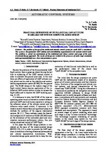
To evaluate the control performance of the CL algorithm 10 different runs of 50000 iterations using random trajectories were done. The performance reached after each run is evaluated using a reference trajectory composed of 20 sigma-shaped randomly generated subtrajectories of different duration and angular variation (figure 2). Reference Trajectory

θ

G

n=100

1

θ (rad)

M

τ Figure 1: Manipulator.

0 -1

Model equations are (Craig, 1989):

where Volt is the input voltage and θ is the angular position. The simulation is made considering a dt of 1 (ms). The sample frequency is 50 (ms). In order to evaluate the CL algorithm we compare the results obtained with a control performed by a PID system tuned using the second method of the Ziegler-Nichols rule (Ogata, 2002).

3.1 CL Algorithm Formulation To make a fair comparison, we use the same input information as in the PID system: the angular position error, the angular velocity error, and the integral of the angular position error. As in Q-learning a discretized representation of the world is needed (Sutton, 1998) (Table 1). Position error eθ near the 0 value is discretized more finely and is denoted by eθ0.

eθ 0

Table 1: Features and actions Range min Range max -π/8 π/8

Features 22

eθ

-π/2

π/2

22

eθ&

-5

5

22

∫ eθ

-100π2

100π2

22

Volt

-48

48

17

0

MSE = 3.226E-3 (rad2)

-0.2 0.2

CL Algorithm Control Error

0

-0.2

MSE = 1.488E-3 (rad2) 0

10

20

30

40

50

60

70

time (s) Figure 2: Instantaneous errors, in larger scale, of the controls performed by the CL algorithm with minimum MSE and the PID.

The mean squared error (MSE) of the control performed by the PID system over the reference trajectory is 3.226E-3 (rad2). The average MSE of the experiments is 2.704E-3 (rad2). This is a remarkable result considering that the CL algorithm uses discretized variables with a reduced number of segments against the continuous variables used by the PID system. This fact causes the low amplitude ripple present in the CL algorithm control. As shown in figure 3, the CL algorithm presents a fast learning convergence, obtaining an acceptable control performance at early stages of the learning process (in about 15000 iterations, 12 minutes of real simulation time). 0

Experiments average reward

-0.5

Our goal is to follow the reference trajectory as close as possible. A natural reward function is:

ra (t ) = − eθ

PID Control Error

reward

Detector

eθ (rad)

(6)

Ri = Volt − nK M θ&

0.2

eθ (rad)

(n 2 J R + ml 2 )θ&& + nM R sign(θ&) + mlG cos(θ ) = K M i (5)

(7)

-1

-1.5

0

1

2

3

4

5x104

iterations Figure 3: Average reward in the 10 experiments performed with the CL algorithm.

In order to illustrate how the algorithm generates relevant partial rules we show in Table 2 the mean number of partial rules generated. To simplify, we only consider their component detectors. Table 2: Mean number of partial rules Detectors Number of rules Order 1 1469

{eθ 0 , eθ& }

2085

{eθ , eθ& }

388

{eθ 0 , ∫ eθ }

269

{eθ , ∫ eθ }

444

{eθ& , ∫ eθ }

58

{eθ 0 , eθ& , ∫ eθ }

2485

{eθ , eθ& , ∫ eθ }

232

Total

7457

The number of rules generated is very low compared with the total number of possible situations, about 362E3, showing the high generalization reached. The CL algorithm is capable to learn that the position error is very relevant for the control task generating rules contain this feature. The CL algorithm was capable to generate partial rules containing the velocity error in regions of the state space near the reference trajectory in which this detector becomes relevant.

5

CONCLUSIONS

In this work we presented a learning approach that uses a new kind of generalization, which we called categorization. The application of this learning system compares well with traditional control techniques, and even outperforms them. The CL algorithm can reach a high generalization with fast learning convergence. This illustrates the viability of its application for complex control. The next step will be the application of continuous domain methods in the CL algorithm expecting to overcome the existing problems of automatic learning in complex control tasks.

ACKNOWLEDGEMENTS This work has been partially supported by the Ministerio de Ciencia y Tecnología and FEDER,

under the project DPI2003-05193-C02-01 of the Plan Nacional de I+D+I.

REFERENCES Agostini, A., Celaya, E., 2004a. Learning in Complex Environments with Feature-Based Categorization. In Proc. of 8th Conference on Intelligent Autonomous Systems. Amsterdam, The Netherland, pp. 446-455. Agostini, A., Celaya, E., 2004b. Trajectory Tracking Control of a Rotational Joint using Feature Based Categorization Learning. In Proc. of IEEE/RSJ International Conference on Intelligent Robots and Systems. Sendai, Japan, pp. 3489-3494. Blom, G., 1989. Probability and Statistics: Theory and Applications. The book. Springer-Verlag. Craig, J., 1989. Introduction to Robotics. The book, 2nd Ed. Addison-Wesley Publishing Company. Grossberg, S., 1982. A Psychophysiological Theory of Reinforcement, Drive, Motivation and Attention. Journal of Theoretical Neurobiology, 1, 286 369. Martins-Filho, L., Silvino, j., Presende, P., Assunçao, T., 2003. Control of robotic leg joints – comparing PD and sliding mode approaches. In Proc. of the Sixth International Conference on Climbing and Walking Robots (CLAWAR2003). Catania, Italy, pp.147-153. Maxon Motor (n. d.). High Precision Drives and Systems. Maxon Interelectric AG, Switzerland. From Maxon Motor Web site http://www.maxonmotor.com. Ogata, K., 2002. Modern Control Engineering. The book. 4th ed., Prentice Hall, New Jersey, United State. Porta, J. M. and Celaya, E., 2000. Learning in Categorizable Environments. In Proc. of the Sixth International Conference on the Simulation of Adaptive Behavior (SAB2000). Paris, pp.343-352. Smart, W. and Kaelbling, L., 2000. Practical reinforcement learning in continuous spaces. In Proc. of the Seventeenth International Conference on Machine Learning (ICML). Sutton, R. and Barto, 1998. Reinforcement Learning. An Introduction. The book. MIT Press. Thrun, S. and Schwartz, A., 1993. Issues in Using Function Approximation for Reinforcement Learning. In Proc. of the Connectionist Models Summer School. Hillsdale, NJ, pp. 255-263. Tsitsikilis, J. and Van Roy, B., 1997. An Analysis of Temporal Difference Learning with Function Approximation. IEEE Transactions on Automatic Control, 42(5):674--690. Watkins, C., Dayan, P., 1992. Q-Learning. Machine Learning, 8:279-292.