Feature-based Similarity Search in Graph Structures - CiteSeerX

Feature-based Similarity Search in Graph Structures Xifeng Yan University of Illinois at Urbana-Champaign Feida Zhu University of Illinois at Urbana-Champaign Philip S. Yu IBM T. J. Watson Research Center and Jiawei Han University of Illinois at Urbana-Champaign Similarity search of complex structures is an important operation in graph-related applications since exact matching is often too restrictive. In this article, we investigate the issues of substructure similarity search using indexed features in graph databases. By transforming the edge relaxation ratio of a query graph into the maximum allowed feature misses, our structural filtering algorithm can filter graphs without performing pairwise similarity computation. It is further shown that using either too few or too many features can result in poor filtering performance. Thus the challenge is to design an effective feature set selection strategy that could maximize the filtering capability. We prove that the complexity of optimal feature set selection is Ω(2m ) in the worst case, where m is the number of features for selection. In practice, we identify several criteria to build effective feature sets for filtering, and demonstrate that combining features with similar size and selectivity can improve the filtering and search performance significantly within a multi-filter composition framework. The proposed feature-based filtering concept can be generalized and applied to searching approximate non-consecutive sequences, trees, and other structured data as well. Categories and Subject Descriptors: H.2.4 [Database Management]: Systems – Query process-

This is a preliminary release of an article accepted by ACM Transactions on Database Systems. The definitive version is currently in production at ACM and, when released, will supersede this version. Authors’ address: X. Yan, F. Zhu, Department of Computer Science, University of Illinois at Urbana-Champaign, Urbana, IL 61801, Email: xyan, [email protected]; P. S. Yu, IBM T. J. Watson Research Center, Hawthorne, NY 10532, Email: [email protected]; J. Han, Department of Computer Science, University of Illinois at Urbana-Champaign, Urbana, IL 61801, Email: [email protected]. Permission to make digital/hard copy of all or part of this material without fee for personal or classroom use provided that the copies are not made or distributed for profit or commercial advantage, the ACM copyright/server notice, the title of the publication, and its date appear, and notice is given that copying is by permission of the ACM, Inc. To copy otherwise, to republish, to post on servers, or to redistribute to lists requires prior specific permission and/or a fee. Request permissions from Publications Dept, ACM Inc., fax +1 (212) 869-0481, or [email protected]. c 2006 ACM 0362-5915/2006/0300-0001 $5.00 ° ACM Transactions on Database Systems, Vol. V, No. N, June 2006, Pages 1–0??.

2

·

Xifeng Yan et al.

ing, Physical Design; G.2.1 [Discrete Mathematics]: Combinatorics – Combinatorial algorithms General Terms: Algorithms, Experimentation, Performance Additional Key Words and Phrases: Graph Database, Similarity Search, Index, Complexity

1.

INTRODUCTION

Development of scalable methods for the analysis of large graph data sets, including graphs built from chemical structures and biological networks, poses great challenges to database research. Due to the complexity of graph data and the diversity of their applications, graphs are generally key entities in widely used databases in chem-informatics and bioinformatics, such as PDB [Berman et al. 2000] and KEGG [Kanehisa and Goto 2000]. In chemistry, the structures and properties of newly discovered or synthesized chemical molecules are studied, classified, and recorded for scientific and commercial purposes. ChemIDplus1 , a free data service offered by the National Library of Medicine (NLM), provides access to structure and nomenclature information. Users can query molecules by their names, structures, toxicity, and even weight in a flexible way through its web interface. Given a query structure, it can quickly identify a small subset of molecules for further analysis [Hagadone 1992, Willett et al. 1998], thus shortening the discovery cycle in drug design and other scientific activities. Nevertheless, the usage of a graph database as well as its query system is not confined to chemical informatics only. In computer vision and pattern recognition [Petrakis and Faloutsos 1997, Messmer and Bunke 1998, Beretti et al. 2001], graphs are used to represent complex structures such as hand-drawn symbols, fingerprints, 3D objects, and medical images. Researchers extract graph models from various objects and compare them to identify unknown objects and scenes. The developments in bioinformatics also call for efficient mechanisms in querying a large number of biological pathways and protein interaction networks. These networks are usually very complex with multi-level structures embedded [Kanehisa and Goto 2000]. All of these applications indicate the importance and the broad usage of graph databases and its accompanying similarity search system. While the motif discovery in graph datasets has been studied extensively, a systematic examination of graph query is becoming equally important. A major kind of query in graph databases is searching topological structures, which cannot be answered efficiently using existing database infrastructures. The indices built on the labels of vertices or edges are usually not selective enough to distinguish complicated, interconnected structures. Due to the limitation of processing graph queries using existing database techniques, tremendous efforts have been put into building practical graph query systems. Most of them fall into the following three categories: (1) full structure search: find structures exactly the same as the query graph [Beretti et al. 2001]; (2) substructure search: find structures that contain the query graph, or vice versa [Shasha et al. 2002, Srinivasa and Kumar 2003, Yan et al. 2004]; and (3) full structure sim1 http://chem.sis.nlm.nih.gov/chemidplus.

ACM Transactions on Database Systems, Vol. V, No. N, June 2006.

Feature-based Similarity Search in Graph Structures

·

3

ilarity search: find structures that are similar to the query graph [Petrakis and Faloutsos 1997, Willett et al. 1998, Raymond et al. 2002]. These kinds of queries are very useful. For example, in substructure search, a user may not know the exact composition of the full structure he wants, but requires that it contain a set of small functional fragments. A common problem in substructure search is: what if there is no match or very few matches for a given query graph? In this situation, a subsequent query refinement process has to be taken in order to find the structures of interest. Unfortunately, it is often too time-consuming for a user to perform manual refinements. One solution is to ask the system to find graphs that nearly contain the entire query graph. This similarity search strategy is more appealing since the user can first define the portion of the query for exact matching and let the system change the remaining portion slightly. The query could be relaxed progressively until a relaxation threshold is reached or a reasonable number of matches are found. N N

O N N

N

N

O

O

N

N

O

O

N

N N

N

N N

O

(a) caffeine

S O

O

(b) thesal Fig. 1.

(c) viagra

A Chemical Database

N

N

N N

O

Fig. 2.

A Query Graph

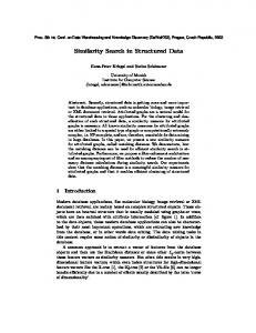
Example 1. Figure 1 is a chemical dataset with three molecules. Figure 2 shows a substructure query. Obviously, no match exists for this query graph. If we relax the query with one edge miss, caffeine and thesal in Figures 1(a) and 1(b) will be good matches. If we relax the query further, the structure in Figure 1(c) could also be an answer. Unfortunately, few systems are available for this kind of search scheme in large scale graph databases. Existing tools such as ChemIDplus only provide the full structure similarity search and the exact substructure search. Other studies usually focus on how to compute the substructure similarity between two graphs efficiently [Nilsson 1980]. This leads to the linear complexity with respect to the size of graph database since each graph in the database has to be checked. ACM Transactions on Database Systems, Vol. V, No. N, June 2006.

4

·

Xifeng Yan et al.

Given that the pairwise substructure similarity computation is very expensive, practically it is not affordable in a large database. A na¨ıve solution is to form a set of subgraph queries with one or more edge misses and then use the exact substructure search. This does not work well even when the number of misses is slightly higher than 1. For example, ¡ if¢ we allow three edges to be missed in a 20edge query graph, it may generate 20 3 = 1, 140 substructure queries, which is too expensive to check. Therefore, a better solution is greatly preferred. In this article, we propose a feature-based structural filtering algorithm, called Grafil (Graph Similarity Filtering), to perform substructure similarity search in a large scale graph database. Grafil models each query graph as a set of features and transforms edge misses into feature misses in the query graph. With an upper bound on the maximum allowed feature misses, Grafil can filter many graphs directly without performing pairwise similarity computations. As a filtering technology, Grafil will improve the performance of existing pairwise substructure similarity search systems as well as the na¨ıve approach discussed above in large graph databases. To facilitate the feature-based filtering, we introduce two data structures, featuregraph matrix and edge-feature matrix. The feature-graph matrix, initially proposed by Giugno and Shasha [Giugno and Shasha 2002, Shasha et al. 2002], is an index structure to compute the difference in the number of features between a query graph and graphs in the database. The edge-feature matrix is built on the fly to compute a bound on the maximum allowed feature misses based on a query relaxation ratio. It will be shown here that using too many features will not improve the filtering performance due to a frequency conjugation phenomenon identified through our study. This counterintuitive result inspires us to identify better combinations of features for filtering purposes. A geometric interpretation is thus proposed to capture the rationale behind the frequency conjugation phenomenon, which also deepens our understanding of the complexity of optimal feature set selection. We prove that it takes Ω(2m ) steps to find an optimal solution in the worst case, where m is the number of features for selection. Practically, we develop a multi-filter composition strategy, where each filter uses a distinct and complementary subset of the features. The filters are constructed by a hierarchical, one-dimensional clustering algorithm that groups features with similar selectivity into a feature set. The experimental result shows that the multi-filter strategy can improve performance significantly for a moderate relaxation ratio. To the best of our knowledge, there is no previous work using feature clustering to improve the filtering performance. A significant contribution of this study is an examination of an increasingly important search problem in graph databases and a new perspective into handling the graph similarity search: instead of indexing approximate substructures, we propose a feature-based indexing and filtering framework, which is a general model that can be applied to searching approximate, non-consecutive sequences, trees, and other complicated structures as well. The rest of the article is organized as follows. Related work is presented in Section 2. Section 3 defines the preliminary concepts. We introduce our structural filtering technique in Section 4, followed by an exploration of optimal feature set selection, its complexity and the development of clustering-based feature selection in Section ACM Transactions on Database Systems, Vol. V, No. N, June 2006.

Feature-based Similarity Search in Graph Structures

·

5

5. Section 6 describes the algorithm implementation, while our performance study is reported in Section 7. Section 8 concludes our study. 2.

RELATED WORK

Structure similarity search has been studied in various fields. Willett et al. [Willett et al. 1998] summarized the techniques of fingerprint-based and graph-based similarity search in chemical compound databases. Raymond et al. [Raymond et al. 2002] proposed a three-tier algorithm for full structure similarity search. Recently, substructure search has attracted lots of attention in the database research community. Shasha et al. [Shasha et al. 2002] developed a path-based approach for substructure search, while Srinivasa et al. [Srinivasa and Kumar 2003] built multiple abstract graphs for the indexing purpose. Yan et al. [Yan et al. 2004] took the discriminative frequent structures as indexing features to improve the search performance. As to substructure similarity search, in addition to graph edit distance and alignment distance, maximum common subgraph is used to measure the similarity between two structures. Unfortunately, finding the maximum common subgraph is NP-complete [Garey and Johnson 1979]. Nilsson[Nilsson 1980] presented an algorithm for the pairwise approximate substructure matching. The matching is greedily performed to minimize a distance function for two structures. Hagadone [Hagadone 1992] recognized the importance of substructure similarity search in a large set of graphs. He used the atom and edge label to do screening. Holder et al. [Holder et al. 1994] adopted the principle of minimum description length for approximate graph matching. Messmer and Bunke [Messmer and Bunke 1998] studied the reverse substructure similarity search problem in computer vision and pattern recognition. These methods did not explore the potential of using more complicated structures to improve the filtering performance, which is studied extensively by our work. In [Shasha et al. 2002], Shasha et al. also extended their substructure search algorithm to support queries with wildcards, i.e., don’t care nodes and edges. Different from their similarity model, we do not fix the positions of wildcards, thus allowing a general and flexible search scheme. In our recent work [Yan et al. 2005], we introduced the basic concept of a featurebased indexing and filtering methodology for substructure similarity search. It was shown that using either too few or too many features can result in poor filtering performance. In this extended work, we provide a geometric interpretation to this phenomena, followed by a rigorous analysis on the feature set selection problem using a linear inequality system. We propose three optimization problems in our filtering framework and prove that each of them takes Ω(2m ) steps to find the optimal solution in the worst case, where m is the number of features for selection. These results ask for selection heuristics, such as clustering-based feature set selection developed in our solution. Besides the full-scale graph search problem, researchers also studied the approximate tree search problem. Wang et al. [Wang et al. 1994] designed an interactive system that allows a user to search inexact matchings of trees. Kailing et al. [Kailing et al. 2004] presented new filtering methods based on tree height, node degree and label information. ACM Transactions on Database Systems, Vol. V, No. N, June 2006.

6

·

Xifeng Yan et al.

The structural filtering approach presented in this study is also related to string filtering algorithms. A comprehensive survey on various approximate string filtering methods was presented by Navarro [Navarro 2001]. The well-known q-gram method was initially developed by Ullmann [Ullmann 1977]. Ukkonen [Ukkonen 1992] independently discovered the q-gram approach, which was further extended in [Gravano et al. 2001] against large scale sequence databases. These q-gram algorithms work for consecutive sequences, not structures. Our work generalized the q-gram method to fit structural patterns of various sizes. 3.

PRELIMINARY CONCEPTS

Graphs are widely used to represent complex structures that are difficult to model. In a labeled graph, vertices and edges are associated with attributes, called label s. The labels could be tags in XML documents, atoms and bonds in chemical compounds, genes in biological networks, and object descriptors in images. The choice of using labeled graphs or unlabeled graphs depends on the application need. The filtering algorithm we proposed in this article can handle both types efficiently. Let V (G) denote the vertex set of a graph G and E(G) the edge set. A label function, l, maps a vertex or an edge to a label. The size of a graph is defined by the number of edges it has, written as |G|. A graph G is a subgraph of G′ if there exists a subgraph isomorphism from G to G′ , denoted by G ⊆ G′ , in which case it is called a supergraph of G. Definition 1 Subgraph Isomorphism. A subgraph isomorphism is an injective function f : V (G) → V (G′ ), such that (1) ∀u ∈ V (G), f (u) ∈ V (G′ ) and l(u) = l′ (f (u)), and (2) ∀(u, v) ∈ E(G), (f (u), f (v)) ∈ E(G′ ) and l(u, v) = l′ (f (u), f (v)), where l and l′ is the label function of G and G′ , respectively. Such a function f is called an embedding of G in G′ . Given a graph database and a query graph, we may not find a graph (or may find only a few graphs) in the database that contains the whole query graph. Thus, it would be interesting to find graphs that contain the query graph approximately, which is a substructure similarity search problem. Based on our observation, this problem has two scenarios, similarity search and reverse similarity search. Definition 2 Substructure Similarity Search. Given a graph database D = {G1 , G2 , . . . , Gn } and a query graph Q, similarity search is to discover all the graphs that approximately contain this query graph. Reverse similarity search is to discover all the graphs that are approximately contained in this query graph. Each type of search scenario has its own applications. In chemical informatics, similarity search is more popular, while reverse similarity search has key applications in pattern recognition. In this article, we develop a structural filtering algorithm for similarity search. Nevertheless, our algorithm can also be applied to reverse similarity search with slight modifications. To distinguish a query graph from the graphs in a database, we call the latter target graphs. The question is how to measure the substructure similarity between a target graph and the query graph. There are several similarity measures. We can classify them into three categories: (1) physical property-based, e.g., toxicity and weight; (2) feature-based; and (3) structure-based. For the feature-based measure, ACM Transactions on Database Systems, Vol. V, No. N, June 2006.

Feature-based Similarity Search in Graph Structures

·

7

domain-specific elementary structures are first extracted as features. Whether two graphs are similar is determined by the number of common features they have. For example, we can compare two compounds based on the number of benzene rings they have. Under this similarity definition, each graph is represented as a feature vector, x = [x1 , x2 , . . . , xn ]T , where xi is the frequency of feature fi . The distance between two graphs is measured by the distance between their feature vectors. Because of its efficiency, the feature-based similarity search has become a standard retrieval mechanism [Willett et al. 1998]. However, the feature-based approach only provides a very rough measure on structure similarity since it loses the global structural connectivity. Sometimes it is hard to build an “elementary structure” dictionary for a graph database, due to the lack of domain knowledge. In contrast, the structure-based similarity measure directly compares the topology of two graphs, which is often costly to compute. However, since this measure takes structure connectivity fully into consideration, it is more accurate than the feature-based measure. Bunke and Shearer [Bunke and Shearer 1998] used the maximum common subgraph to measure full structure similarity. Researchers also developed the concept of graph edit distance by simulating the graph matching process in a way similar to the string matching process (akin to string edit distance). No matter what the definition is, the matching of two graphs can be regarded as a result of three edit operations: insertion, deletion, and relabeling. According to the substructure similarity search, each of these operations relaxes the query graph by removing or relabeling one edge (insertion does not change the query graph). Thus, we take the percentage of retained edges in the query graph as a similarity measure. Definition 3 Relaxation Ratio. Given two graphs G and Q, if P is the maximum common subgraph2 of G and Q, then the substructure similarity between G |E(P )| |E(P )| and Q is defined by |E(Q)| , and 1 − |E(Q)| is called relaxation ratio. Example 2. Consider the target graph in Figure 1(a) and the query graph in Figure 2. Their maximum common subgraph has 11 out of the 12 edges. Thus, the substructure similarity between these two graphs is around 92% with respect to the query graph. That also means if we relax the query graph by 8%, the relaxed query graph is contained in Figure 1(a). The similarity of graphs in Figures 1(b) and 1(c) with the query graph is 92% and 67%, respectively. With the advance of computational power, it is affordable to compute the maximum common subgraph for two sparse graphs. Nevertheless, the pairwise similarity computation through a large graph database is still time-consuming. In this article, we want to examine how to build a connection between the structure-based measure and the feature-based measure so that we can use the feature-based measure to screen the database before performing expensive pairwise structure-based similarity computation. Using this strategy, we are able to take advantage of both measures: efficiency from the feature-based measure and accuracy from the structure-based measure. 2 The

maximum common subgraph is not necessarily connected. ACM Transactions on Database Systems, Vol. V, No. N, June 2006.

8

4.

·

Xifeng Yan et al.

STRUCTURAL FILTERING

Given a relaxed query graph, the major goal of our algorithm is to filter out as many graphs as possible using a feature-based approach. The features discussed here could be paths [Shasha et al. 2002], discriminative frequent structures [Yan et al. 2004], elementary structures, or any structures indexed in a graph database. Previous work did not investigate the connection between the structure-based similarity measure and the feature-based similarity measure. In this study, we explicitly transform the query relaxation ratio to the number of misses of indexed features, thus building a connection between these two measures. e1

e2

Fig. 3.

(a) f a Fig. 4.

e3

A Sample Query

(b) f b

(c)f

c

A sample set of features

Let us first consider an example. Figure 3 shows a query graph and Figure 4 depicts three structural fragments. Assume that these fragments are indexed as features in a graph database. For simplicity, we ignore all the label information in this example. The symbols e1 , e2 , and e3 in Figure 3 do not represent labels but edges themselves. Suppose we cannot find any match for this query graph in a graph database. Then a user may relax one edge, e1 , e2 , or e3 , through a deletion or relabeling operation. He/she may deliberately retain the middle edge, because the deletion of that edge may break the query graph into pieces. Because the relaxation can take place among e1 , e2 , and e3 , we are not sure which feature will be affected by this relaxation. However, no matter which edge is relaxed, the relaxed query graph should have at least three embeddings of these features. Equivalently, we say that the relaxed query graph may miss at most four embeddings of these features in comparison with the original query graph, which have seven embeddings: one fa , two fb ’s, and four fc ’s. Using this information, we can discard graphs that do not contain at least three embeddings of these features. We name the above filtering concept feature-based structural filtering. ACM Transactions on Database Systems, Vol. V, No. N, June 2006.

Feature-based Similarity Search in Graph Structures

4.1

·

9

Feature-Graph Matrix Index

In order to facilitate the feature-based filtering, we need an index structure, referred to as the feature-graph matrix [Giugno and Shasha 2002, Shasha et al. 2002]. Each column of the feature-graph matrix corresponds to a target graph in the graph database, while each row corresponds to a feature being indexed. Each entry records the number of the embeddings of a specific feature in a target graph. Suppose we have a sample database with four graphs, G1 , G2 , G3 , and G4 . Figure 5 shows an example. For instance, G1 has two embeddings of fc . The feature-graph matrix index is easily maintainable: as each time a new graph is added to the graph database, only an additional column needs to be added.

G1

G2

G3

G4

fa

0

1

0

0

fb

0

0

1

0

fc

2

3

4

4

Fig. 5.

Feature-Graph Matrix Index

Using the feature-graph matrix, we can apply the feature-based filtering on any query graph against a target graph in the database using any subset of the indexed features. Consider the query shown in Figure 3 with one edge relaxation. According to the feature-graph matrix in Figure 5, even if we do not know the structure of G1 , we can filter G1 immediately based on the features included in G1 , since G1 only has two of all the embeddings of fa , fb , and fc . This feature-based filtering process is not involved with any costly structure similarity checking. The only computation needed is to retrieve the features from the indices that belong to a query graph and compute the possible feature misses for a relaxation ratio. Since our filtering algorithm is fully built on the feature-graph matrix index, we need not access the physical database unless we want to calculate the accurate substructure similarity. We implement the feature-graph matrix based on a list, where each element points to an array representing the row of the matrix. Using this implementation, we can flexibly insert and delete features without rebuilding the whole index. In the next subsection, we will present the general framework of processing similarity search, and illustrate the position of our structural filtering algorithm in this framework. 4.2

A General Framework

Given a graph database and a query graph, the substructure similarity search can be performed within a general framework detailed in the following four steps. (1) Index construction: Select small structures as features in the graph database, and build the feature-graph matrix between the features and the graphs in the database. ACM Transactions on Database Systems, Vol. V, No. N, June 2006.

·

10

Xifeng Yan et al.

(2) Feature miss estimation: Determine the indexed features belonging to the query graph, select a feature set (i.e., a subset of the features), calculate the number of selected features contained in the query graph and then compute the upper bound of feature misses if the query graph is relaxed with one edge deletion or relabeling. This upper bound is written as dmax . Some portion of the query graph can be specified as not to be altered, e.g., key functional structures. (3) Query processing: Use the feature-graph matrix to calculate the difference in the number of features between each graph G in the database and query Q. If the difference is greater than dmax , discard graph G. The remaining graphs constitute a candidate answer set, written as CQ . We then calculate substructure similarity using the existing algorithms and prune the false positives in CQ . (4) Query relaxation: Relax the query further if the user needs more matches than those returned from the previous step; iterate Steps 2 to 4. The feature-graph matrix in Step 1 is built beforehand and can be used by any query. The similarity search for a query graph takes place in Step 2 and Step 3. The filtering algorithm proposed should return a candidate answer set as small as possible since the cost of the accurate similarity computation is proportional to the size of the candidate set. Quite a lot of work has been done at calculating the pairwise substructure similarity. Readers are referred to the related work in [Nilsson 1980, Hagadone 1992, Raymond et al. 2002]. In the step of feature miss estimation, we calculate the number of features in the query graph. One feature may have multiple embeddings in a graph; thus, we use the number of embeddings of a feature as a more precise term. In this article, these two terms are used interchangeably for convenience. In the rest of this section, we will introduce how to estimate feature misses by translating it into the maximum coverage problem. The estimation is further refined through a branch-and-bound method. In Section 5, we will explore the opportunity of using different feature sets to improve filtering efficiency. 4.3

Feature Miss Estimation

Substructure similarity search is akin to approximate string matching. In approximate string matching, filtering algorithms such as q-gram achieve the best performance because they do not inspect all the string characters. However, filtering algorithms only work for a moderate relaxation ratio and need a validation algorithm to check the actual matches [Navarro 2001]. Similar arguments also apply to our structural filtering algorithm in substructure similarity search. Fortunately, since we are doing substructure search instead of full structure similarity search, usually the relaxation ratio is not very high in our problem setting. A string with q characters is called a q-gram. A typical q-gram filtering algorithm builds an index for all q-grams in a string database. A query string Q is broken into a set of q-grams, which are compared against the q-grams of each target string in the database. If the difference in the number of q-grams is greater than the following threshold, Q will not match this string within k edit distance. Given two strings P and Q, if their edit distance is k, their difference in the ACM Transactions on Database Systems, Vol. V, No. N, June 2006.

Feature-based Similarity Search in Graph Structures

·

11

number of q-grams is at most kq [Ukkonen 1992]. It would be interesting to check whether we can similarly derive a bound for size-q substructures. Unfortunately, we may not draw a succinct bound like the one given to q-grams due to the following two issues. First, in substructure similarity search, the space of size-q subgraphs is exponential with respect to q. This contrasts with the string case where the number of q-grams in a string is linear to its length. Secondly, even if we index all of the size-q subgraphs, the above q-gram bound will not be valid since the graph does not have the linearity that the string does.

f a f b(1) f b(2) f c(1) f c(2) f c(3) f c(4) e1

0

1

1

1

0

0

0

e2

1

1

0

0

1

0

1

e3

1

0

1

0

0

1

1

Fig. 6.

Edge-Feature Matrix

In order to calculate the maximum feature misses for a given relaxation ratio, we introduce edge-feature matrix that builds a map between edges and features for a query graph. In this matrix, each row represents an edge while each column represents an embedding of a feature. Figure 6 shows the matrix built for the query graph in Figure 3 and the features shown in Figure 4. All of the embeddings are recorded. For example, the second and the third columns are two embeddings of feature fb in the query graph. The first embedding of fb cover s edges e1 and e2 while the second covers edges e1 and e3 . The middle edge does not appear in the edge-feature matrix if a user prefers retaining it. We say that an edge ei hits a feature fj if fj covers ei . It is not expensive to build the edge-feature matrix on the fly as long as the number of features is small. Whenever an embedding of a feature is discovered, a new column is attached to the matrix. We formulate the feature miss estimation problem as follows: Given a query graph Q and a set of features contained in Q, if the relaxation ratio is θ, what is the maximum number of features that can be missed ? In fact, it is the maximum number of columns that can be hit by k rows in the edge-feature matrix, where k = ⌊θ ·|G|⌋. This is a classic maximum coverage (or set k-cover) problem, which has been proved NP-complete. The optimal solution that finds the maximal number of feature misses can be approximated by a greedy algorithm. The greedy algorithm first selects a row that hits the largest number of columns and then removes this row and the columns covering it. This selection and deletion operation is repeated until k rows are removed. The number of columns removed by this greedy algorithm provides a way to estimate the upper bound of feature misses. Algorithm 1 shows the pseudo-code of the greedy algorithm. Let mrc be the entry in the r-th row, c-th column of matrix M. Mr denotes the r-th row vector of matrix M, while Mc denotes the c-th column vector of matrix M. |Mr | represents the ACM Transactions on Database Systems, Vol. V, No. N, June 2006.

12

·

Xifeng Yan et al.

number of non-zero entries in the r-th row. Line 3 in Algorithm 1 returns the row with the maximum number of non-zero entries. Algorithm 1 GreedyCover Input: Edge-feature Matrix M, Maximum edge relaxations k. Output: The number of feature misses Wgreedy . 1: let Wgreedy = 0; 2: for each l = 1 . . . k do 3: select row r s.t. r = arg maxi |Mi |; 4: Wgreedy = Wgreedy + |Mr |; 5: for each column c s.t. mrc = 1 do 6: set Mc =0; 7: return Wgreedy ;

Theorem 1. Let Wgreedy and Wopt be the total feature misses computed by the greedy solution and by the optimal solution. We have 1 k 1 ) ] Wopt ≥ (1 − ) Wopt , k e where k is the number of edge relaxations. Wgreedy ≥ [1 − (1 −

(1)

Proof. [Hochbaum 1997] It can be shown theoretically that the optimal solution cannot be approximated in polynomial time within a ratio of (e/(e − 1) − o(1)) unless P = NP [Feige 1998]. We rewrite the inequality in Theorem 1. 1 Wgreedy 1 − (1 − k1 )k e Wgreedy ≤ e−1 ≤ 1.6 Wgreedy

Wopt ≤ Wopt Wopt

(2)

Traditional applications of the maximum coverage problem focus on how to approximate the optimal solution as much as possible. Here we are only interested in the upper bound of the optimal solution. Let maxi |Mi | be the maximum number of features that one edge hits. Obviously, Wopt should be less than k times of this number, Wopt ≤ k × max |Mi |. i

(3)

The above bound is actually adopted from q-gram filtering algorithms. This bound is a bit loose in our problem setting. The upper bound derived from Inequality 2 is usually tighter for non-consecutive sequences, trees and other complex ACM Transactions on Database Systems, Vol. V, No. N, June 2006.

Feature-based Similarity Search in Graph Structures

·

13

structures. It may also be useful for approximate string filtering if we do not enumerate all q-grams in strings for a given query string. 4.4

Estimation Refinement

A tight bound of Wopt is critical to the filtering performance since it often leads to a small set of candidate graphs. Although the bound derived by the greedy algorithm cannot be improved asymptotically, we may still improve the greedy algorithm in practice. Let Wopt (M, k) be the optimal value of the maximum feature misses for k edge relaxations. Suppose r = arg maxi |Mi |. Let M′ be M except (M′ )r = 0 and (M′ )c = 0 for any column c that is hit by row r, and M′′ be M except (M′′ )r = 0. Any optimal solution that leads to Wopt should satisfy one of the following two cases: (1) r is selected in this solution; or (2) r is not selected (we call r disqualified for the optimal solution). In the first case, the optimal solution should also contain the optimal solution for the remaining matrix M′ . That is, Wopt (M, k) = |Mr | + Wopt (M′ , k − 1). k − 1 means that we need to remove the remaining k − 1 rows from M′ since row r is selected. In the second case, the optimal solution for M should be the optimal solution for M′′ , i.e., Wopt (M, k) = Wopt (M′′ , k). k means that we still need to remove k rows from M′′ since row r is disqualified. We call the first case the selection step, and the second case the disqualifying step. Since the optimal solution is to find the maximum number of columns that are hit by k edges, Wopt should be equal to the maximum value returned by these two steps. Therefore, we can draw the following conclusion. Lemma 1. ( |Mr | + Wopt (M′ , k − 1), Wopt (M, k) = max Wopt (M′′ , k).

(4)

Lemma 1 suggests a recursive solution to calculate Wopt . It is equivalent to enumerating all the possible combinations of k rows in the edge-feature matrix, which may be very costly. However, it is worth exploring the top levels of this recursive process, especially for the case where most of the features intensively cover a set of common edges. For each matrix M′ (or M′′ ) that is derived from the original matrix M after several recursive calls in Lemma 1, M′ encountered interleaved selection steps and disqualifying steps. Suppose M′ has h selected rows and b disqualified rows. We restrict h to be less than H and b to be less than B, where H and B are predefined constants, and H + B should be less than the number of rows in the edge-feature matrix. In this way, we can control the depth of the recursion. Let Wapx (M, k) be the upper bound on the maximum feature misses calculated using Equations (2) and (3), where M is the edge-feature matrix and k is the number of edge relaxations. We formulate the above discussion in Algorithm 2. Line 7 selects row r while Line 8 disqualifies row r. Lines 7 and 8 correspond to the selection and disqualifying steps shown in Lemma 1. Line 9 calculates the maximum value of the result returned by Lines 7 and 8. Meanwhile, we can also use the greedy algorithm to get the upper bound of Wopt directly, as Line 10 does. Algorithm 2 returns the best estimation we can get. The condition in Line 1 will terminate the ACM Transactions on Database Systems, Vol. V, No. N, June 2006.

14

·

Xifeng Yan et al.

recursion when it selects H rows or when it disqualifies B rows. Algorithm 2 is a classical branch-and-bound approach.

Algorithm 2 West (M, k, h, b) Input: Edge-feature Matrix M, Number of edge relaxations k, h selection steps and b disqualifying steps. Output: Maximum feature misses West . 1: if b ≥ B or h ≥ H then 2: return Wapx (M, k); 3: select row r that maximizes |Mr |; 4: let M′ = M and M′′ = M; 5: set (M′ )r = 0 and (M′ )c = 0 for any c if mrc = 1; 6: set (M′′ )r = 0; 7: W1 = |Mr | + West (M′ , k − 1, h + 1, b) ; 8: W2 = West (M′′ , k, h, b + 1) ; 9: Wa = max(W1 , W2 ) ; 10: Wb = Wapx (M, k); 11: return West = min(Wa , Wb );

We select parameters H and B such that H is less than the number of edge relaxations, and H + B is less than the number of rows in the matrix. Algorithm 2 is initialized by West (M, k, 0, 0). The bound obtained by Algorithm 2 is not greater than the bound derived by the greedy algorithm since we intentionally select the smaller one in Lines 10-11. On the other hand, West (M, k, 0, 0) is not less than the optimal value since Algorithm 2 is just a simulation of the recursion in Lemma 1, and at each step, it has a greater value. Therefore, we can draw the following conclusion. Lemma 2. Given two non-negative integers H and B in the branch-and-bound algorithm (Algorithm 2), if H ≤ k and H + B ≤ n, where k is the number of edge relaxations and n is the number of rows in the edge-feature matrix M, we have Wopt (M, k) ≤ West (M, k, 0, 0) ≤ Wapx (M, k).

(5)

Proof. Lines 10 and 11 in Algorithm 2 imply that the second inequality is obvious. We prove the first inequality using induction. Let M(h,b) be the matrix derived from M with h rows selected and b rows disqualified. West (M(h,B) , k, h, B) = Wapx (M(h,B) , k) ≥ Wopt (M(h,B) , k) West (M(H,b) , k, H, b) = Wapx (M(H,b) , k) ≥ Wopt (M(H,b) , k) Assume that Wopt (M(h,b) , k) ≤ West (M(h,b) , k, h, b) for some h and b, 0 < h ≤ H and 0 < b ≤ B. Let West (M(h−1,b) , k, h−1, b) = min{max{W1 , W2 }, Wb } according ACM Transactions on Database Systems, Vol. V, No. N, June 2006.

Feature-based Similarity Search in Graph Structures

·

15

to Lines 7-11 in Algorithm 2. Wb = Wapx (M(h−1,b) , k) ≥ Wopt (M(h−1,b) , k) W1 = |Mr | + West (M(h,b) , k − 1, h, b) ≥ |Mr | + Wopt (M(h,b) , k − 1) ≥ Wopt (M(h−1,b) , k) W2 = West (M(h−1,b+1) , k, h − 1, b + 1) ≥ Wopt (M(h−1,b+1) , k) ≥ Wopt (M(h−1,b) , k) Therefore, West (M(h−1,b) , k, h−1, b) ≥ Wopt (M(h−1,b) , k). Similarly, West (M(h,b−1) , k, h, b − 1) ≥ Wopt (M(h,b−1) , k). By induction, Wopt (M, k) ≤ West (M, k, 0, 0). Lemma 2 shows that the bound derived by the branch-and-bound algorithm is between the bounds calculated by the optimal solution and the greedy solution, thus providing a tighter bound on the maximum feature misses. 4.5

Time Complexity

Let us first examine the time complexity of the greedy algorithm shown in Algorithm 1. We maintain the value of |Mr | for all of the rows in an array. Assume that the matrix has n rows and m columns. Line 3 in Algorithm 1 can finish in O(n). Line 4 takes O(1). Line 5 erases columns covering the selected row. When an entry mrc is set at 0, we also update |Mr |. Once an entry is erased, it will not be accessed in the remaining computation. The maximum number of entries to be erased is nm. In each erasing, the value of |Mr | has to be updated for erased entries and the maximum value will be selected for the next-round computation. Therefore, the time complexity of the greedy algorithm is O(nm + kn). Since usually m ≫ k, the complexity can be written as O(nm). Now we are going to examine the time complexity of the branch-and-bound algorithm shown in Algorithm 2. Lemma 3. Given two non-negative integers H and B, TH,B is the number of times that the branch-and-bound algorithm (Algorithm 2) is called. ¶ µ B+H . (6) TH,B = H Proof. We have TH,0 = 1, T0,B = 1, TH,B = TH−1,B + TH,B−1 (Lines 7 and 8). TH,B =

µ

B+H H

¶

is a solution that satisfies the above condition since µ ¶ µ ¶ µ ¶ B+H B+H −1 B+H −1 = + H H −1 H

It takes O(nm) to finish a call to Algorithm 2 if the recursion is excluded. Hence, the time complexity of the branch-and-bound algorithm is O(TH,B · nm). Given ACM Transactions on Database Systems, Vol. V, No. N, June 2006.

16

·

Xifeng Yan et al.

a query Q and the maximum allowed selection and disqualifying steps, H and B, the cost of computing West is irrelevant to the number of the graphs in a database. Thus, the cost of feature miss estimation remains constant with respect to the database size. 4.6

Frequency Difference

Assume that f1 , f2 , . . . , fn form the feature set used for filtering. Once the upper bound of feature misses is obtained, we can use it to filter graphs in our framework. Given a target graph G and a query graph Q, let u = [u1 , u2 , . . . , un ]T and v = [v1 , v2 , . . . , vn ]T be their corresponding feature vectors, where ui and vi are the frequencies (i.e., the number of embeddings) of feature fi in graphs G and Q. Figure 7 shows the two feature vectors u and v. As mentioned before, for any feature set, the corresponding feature vector of a target graph can be obtained from the feature-graph matrix directly without scanning the graph database. u3 u1

u4

u5

u2

Target Graph G

v2 v3 v1 f1

v4 f2

f3

Fig. 7.

f4

v5 Query Graph Q f5

Frequency Difference

We want to know how many more embeddings of feature fi appear in the query graph, compared to the target graph. Equation (7) calculates this frequency difference for feature fi , ( 0, if ui ≥ vi , (7) r(ui , vi ) = vi − ui , otherwise. For the feature vectors shown in Figure 7, r(u1 , v1 ) = 0; we do not take the extra embeddings from the target graph into account. The summed frequency difference of each feature in G and Q is written as d(G, Q). Equation (8) sums up all the frequency differences, d(G, Q) =

n X

r(ui , vi ).

(8)

i=1

Suppose the query can be relaxed with k edges. Algorithm 2 estimates the upper bound of allowed feature misses. If d(G, Q) is greater than that bound, we can conclude that G does not contain Q within k edge relaxations. For this case, we do not need to perform any complicated structure comparison between G and Q. Since all the computations are done on the preprocessed information in the indices, the filtering actually is very fast. ACM Transactions on Database Systems, Vol. V, No. N, June 2006.

Feature-based Similarity Search in Graph Structures

·

17

Before we check the problem of feature selection, let us first examine whether we should include all the embeddings of a feature. An intuition is that we should eliminate the automorphic embeddings of a feature. Definition 4 Graph Automorphism. An automorphism of a graph is a mapping from the vertices of the given graph G back to vertices of G such that the resulting graph is isomorphic with G. Given two feature vectors built from a target graph G and a query graph Q, u = (u1 , u2 , . . . , un ) and v = (v1 , v2 , . . . , vn ), where ui and vi are the frequencies (the number of embeddings) of feature fi in G and Q, respectively. Suppose structure fi has κ automorphisms. Then ui and vi can be divided by κ exactly. It also means that the edge-feature matrix will have duplicate columns. In practice, we should remove these duplicate columns since they do not provide additional information. 5.

FEATURE SET SELECTION

In Section 4, we have explored the basic filtering framework and our bounding technique for feature miss estimation. For a given feature set, the filtering performance could not be improved further unless we have a tighter bound of allowed feature misses. Nevertheless, we have not explored the opportunities of composing filters based on different feature sets. An interesting question is “does a filter achieve good filtering performance if all of the features are used together ?” A seemingly attractive intuition is that the more features are used, the greater pruning power is achieved. After all, we are using more information provided by the query graph. Unfortunately, though a bit counter-intuitive, using all of the features together will not necessarily give the optimal solution; in some cases, it even deteriorates the performance rather than improving it. In the following presentation, we will examine the principles behind this phenomenon and derive the complexity of finding an optimal feature set in the worst case. Given a query graph Q, let F = {f1 , f2 , . . . , fm } be the set of features included in Q, and dkF the maximal number of features missed in F after Q is relaxed (either relabeled or deleted) with k edges. Relabeling and deleting an edge e in Q have the same effect: the features containing e are broken. Let u = [u1 , u2 , . . . , um ]T and v = [v1 , v2 , . . . , vm ]T be the feature vectors built from a target graph G in the graph database and a query graph Q based on a chosen feature set F . Let ΓF = {G|d(G, Q) > dkF }, which is the set of graphs pruned from the index by the feature set F . It is obvious that, for any feature set F , the greater the cardinality of ΓF , the better. In general, a candidate graph G passing a filter should satisfy the following inequality, r(u1 , v1 ) + r(u2 , v2 ) + . . . + r(un , vn ) ≤ dkF . ′

(9) [u′1 , u′2 , . . . , u′n ]T

Let P be the maximum common subgraph of G and Q. Vector u = is its feature vector. If G contains Q within the relaxation ratio, P should contain Q within the relaxation ratio as well, i.e., r(u′1 , v1 ) + r(u′2 , v2 ) + . . . + r(u′n , vn ) ≤ dkF .

(10)

ACM Transactions on Database Systems, Vol. V, No. N, June 2006.

18

·

Xifeng Yan et al.

Since for any feature fi , ui ≥ u′i , we have r(ui , vi ) ≤ r(u′i , vi ), n n X X r(ui , vi ) ≤ r(u′i , vi ). i=1

i=1

Inequality (10) is stronger than Inequality (9). Mathematically, we should check Inequality (10) instead of Inequality (9). However, we do not want to calculate P , the maximum common subgraph of G and Q, beforehand, due to its computational cost. Inequality (9) is the only choice we have. Assume that Inequality (10) does not hold for graph P , and furthermore, there exists a feature fi such that its frequency in P is too small to make Inequality (10) hold. However, we can still make Inequality (9) true for graph G, if we compensate the misses of fi by adding more occurrences of another feature fj in G. We call this phenomenon feature conjugation. Feature conjugation is likely to be taking place in our filtering algorithm since the filtering does not distinguish the misses of a single feature, but a collective set of features. As one can see, because of feature conjugation, we may fail to filter some graphs that do not satisfy the query requirement. Example 3. Assume that we have a graph G that contains the sample query graph in Figure 3 with edge e3 relaxed. In this case, G must have one embedding of feature fb and two embeddings of fc (fb and fc are in Figure 4). However, we may slightly change G such that it does not contain fb but has one more embedding of fc . This is what G4 has in Figure 5 (G4 could contain 4 2-edge fragments that are disconnected with each other). The feature conjugation takes place when the miss of fb is compensated by the addition of one more occurrence of fc . In such a situation, Inequality (9) is still satisfied for G4 , while Inequality (10) may not. However, if we can divide the features in Figure 4 into two groups, we can partially solve the feature conjugation problem. Let group A contain feature fa and fb , and group B contain feature fc only. For any graph containing the query shown in Figure 3 with one edge relaxation (edge e1 , e2 or e3 ), it must have one embedding in Group A. Using this constraint, we can drop G4 in Figure 5 since G4 does not have any embedding of fa or fb . 5.1

Geometric Interpretation

Example 3 implies that the filtering power may be weakened if we deploy all the features in one filter. A feature has filtering power if its frequency in a target graph is less than its frequency in the query graph; otherwise, it does not help the filtering. Unfortunately, a feature that is good for some graph may not be good for other graphs in the database. We are interested in finding optimal filters that can prune as many unqualified graphs as possible. This leads to a natural questions “What is the optimal feature set for pruning? How hard is it to compute the optimal solution? ” Before solving this optimization problem, it is beneficial to look at the geometric interpretation of the feature-based pruning. Given a chosen feature set F = {f1 , f2 , . . . , fm }, each indexed graph G can be viewed as a point in a space of m dimensions whose coordinates are represented by the feature vector u = [u1 , u2 , . . . , um ]T . ACM Transactions on Database Systems, Vol. V, No. N, June 2006.

Feature-based Similarity Search in Graph Structures

·

19

Lemma 4. For any feature set F = {f1 , f2 , . . . , fm }, max{dk{f1 } , dk{f2 } , . . . , dk{fm } } ≤ dkF ≤

m X

dk{fi }

i=1

Proof. For any i, 1 ≤ i ≤ m, since {fi } ⊆ F , by definition we have dk{fi } ≤ dkF . Let ki be the number of features P missed for P feature fi in the solution to dkF . m m k k Obviously, ki ≤ d{fi } ; therefore, dF = i=1 ki ≤ i=1 dk{fi } .

Let us check a specific case where a query graph Q only has two features f1 and f2 . For any target graph G, G ∈ Γ{f1 ,f2 } if and only if d(G, Q) = r(u1 , v1 ) + r(u2 , v2 ) − dk{f1 ,f2 } > 0. The only situation under which this inequality is guaranteed is when G ∈ Γ{f1 } and G ∈ Γ{f2 } since in this case r(u1 , v1 ) − dk{f1 } > 0 and r(u2 , v2 ) − dk{f2 } > 0. It follows from the lemma above that r(u1 , v1 ) + r(u2 , v2 ) − dk{f1 ,f2 } > 0. It is easy to verify that under all other situations, even if G ∈ Γ{f1 } or G ∈ Γ{f2 } , it can still be the case that G 6∈ Γ{f1 ,f2 } . In the worst case, an evil adversary can construct an index such that |Γ{f1 ,f2 } | < min{|Γ{f1 } |, |Γ{f2 } |}. This discussion shows that an algorithm using all features therefore may fail to yield the optimal solution.

v 1 +v 2 -d {f1,f2} v2 v 2 -d {f2}

v 2 -d {f2} v 1 -d {f1}

v 1 -d {f1} v 1

{f 1 }

{f 2 } Fig. 8.

{f

1,

f2 }

Geometric Interpretation

For a given query Q with two features {f1 , f2 }, each graph G in the database can be represented by a point in the plane with coordinates in the form of (u1 , u2 ). Let v = {v1 , v2 } be the feature vector of Q. To select a feature set and then use it to prune the target graphs is equivalent to selecting a halfspace and throwing away all points in the halfspace. Figure 8 depicts three feature selections: {f1 }, {f2 } and {f1 , f2 }. If only f1 is selected, it corresponds to throwing away all points to the left of line u1 = v1 − dk{f1 } . If only f2 is selected, it corresponds to throwing away all points below line u2 = v2 − dk{f2 } . If both f1 and f2 are selected, it corresponds to throwing away all points below line u1 + u2 = v1 + v2 − dk{f1 ,f2 } , points below the line u2 = v2 − dk{f1 ,f2 } , and points to the left of line u1 = v1 − dk{f1 ,f2 } . It is easy to observe that, depending on the distribution of the points, each feature set could have varied pruning power. Note that, by Lemma 4, the line u1 + u2 = v1 + v2 − dk{f1 ,f2 } is always above the point (v1 − dk{f1 } , v2 − dk{f2 } ); it passes the point if and only if when dk{f1 ,f2 } = ACM Transactions on Database Systems, Vol. V, No. N, June 2006.

20

·

Xifeng Yan et al.

dk{f1 } + dk{f2 } . This explains why even applying all the features one after another for pruning does not generally guarantee the optimal solution. Alternatively, we can conclude that, given the set F = {f1 , f2 , . . . , fm } of all features in a query graph Q, the smallest candidate set remained after the pruning is contained in a convex subspace of the m-dimensional feature space. The convex subspace in the example is shown as shaded area in Figure 8. 5.2

Complexity of Optimal Feature Set Selection

The geometric interpretation presented in the previous section offers us not only insight into the intricacy of the problem within a unified model, but also implies lower bounds of its complexity. Let F = {f1 , f2 , . . . , fm } be the set of all features found in query graph Q. There are 2m − 1 different ways to choose a nonempty feature subset of F . Given a chosen feature set Fi = {fi1 , fi2 , . . . , fij }, Fi ⊆ F , to prune the indexed target graphs by Fi is equivalent to pruning the m-dimensional feature space with the halfspace defined by the inequality r(xi1 , vi1 ) + r(xi2 , vi2 ) + . . .+r(xij , vij ) ≥ dkFi . For simplicity of presentation, we first examine the properties of the halfspace defined by xi1 + xi2 + . . . + xij ≥ vi1 + vi2 + . . . + vij − dkFi ,

(11)

which contains the space defined by Inequality 9. In this case, r(xi , vi ) = vi − xi for any selected feature fi . We will later show that all of the following results hold under the original definition of r(xi , vi ). In the pruning, all points lying in this halfspace may survive while others are definitely pruned away. It is evident at this point that, given the set F = {f1 , f2 , . . . , fm } of all features in Q, the way to prune the most graphs is to use every nonempty subset F ′ ⊆ F successively. The optimal solution thus corresponds to the convex subspace which is the intersection of all the 2m − 1 convex subspaces. However, it is infeasible to access the index 2m − 1 times in practice. We therefore seek a feature set with the greatest pruning power. Unfortunately, we prove in the following that the complexity of computing the best feature set is Ω(2m ) in the worst case. Let Ax ≥ b be the inequality system of all these 2m − 1 inequalities derived from F , where A is a (2m − 1) × m matrix, x ∈ Rn and b ∈ Rn are column vectors (n = 2m − 1). Each inequality has the format shown in Inequality (11). Denote by xi the i-th entry of x, bi the i-th entry of b and aij the entry in the i-th row and j-th column of A. We also denote the i-th row and the j-th column of A as Ai and Aj respectively. By construction, A is a 0 − 1 matrix. The i-th row of A corresponds to the chosen feature set Fi ⊆ F ; aij = 1 if and only if feature fj is P selected in Fi . The corresponding bi = fj ∈Fi vj − dkFi . Let χF = {x ∈ Rn : Ax ≥ b} be the convex subspace containing all the points that survived the pruning by F . We also call χF the feasible region from now on. We prove that there exist query graphs such that none of the inequalities in Ax ≥ b is a redundant constraint, i.e., all the supporting halfplanes appear in the lower envelope of χF . Intuitively, this means that, if we start with the entire m-dimensional feature space and compute the feasible region by adding all the inequalities in Ax ≥ b one after another (in any order), every halfplane defined by an inequality would “cut” off a polytope of nonempty volume from the current ACM Transactions on Database Systems, Vol. V, No. N, June 2006.

Feature-based Similarity Search in Graph Structures

·

21

feasible region. In order to prove this result, we cite the following theorem which is well-known in linear programming. Theorem 2. [Padberg 1995] An inequality dx ≥ d0 is redundant relative to a system of n linear inequalities in m unknowns: Ax ≥ b, x ≥ 0 if and only if the inequality system is unsolvable or there exists a row vector u ∈ Rn satisfying u ≥ 0, d ≥ uA, ub ≥ d0 w(s n )

sn w(s 2 ) w(s 1 ) f1 f2

s2

...

s1

s3

w(s 3 )

...

fm

Fig. 9.

Weighted Set System

Denote as π(X) the set of nonzero indices of a vector X and 2S the power set of S. Lemma 5. Given a graph Q, a feature set F = {f1 , f2 , . . . , fm } (fi ⊆ Q) and a weighted set system Φ = (I, w), where I ⊆ 2F \ {∅, F }, w : I 7→ R+ , define function gΦ : F 7→ R+ , S ½ 0 if f ∈S,S∈I = ∅ gΦ (f ) = P otherwise f ∈S,S∈I w(S)

Denote as gΦ (F ) the feature set F weighted by gΦ such that deleting an edge of a feature f kills an amount of gΦ (f ) of that feature. Let dkgΦ (F ) be the maximum amount of features that can be killed by deleting k edges on Q, for a weighted feature set gΦ (F ). Then, X¡ ¢ max{w(S)dkS } ≤ dkgΦ (F ) ≤ w(S)dkS S∈I

S∈I

Proof. (1) For any S ∈ I, since S ⊆ F , we have dkS ≤ dkF , so the weighted inequality w(S)dkS ≤ w(S)dkF ≤ dkgΦ (F ) . (2) Let F ∗ ⊆ F be the set of features killed in a solution of dkgΦ (F ) . Then for any T S ∈ I,we have |F ∗ ∩ S| ≤ dkS since all features in F ∗ S can be hit by deleting k edges over the feature set S. Summing over I, X X¡ ¢ w(S)dkS ≥ (w(S)|F ∗ ∩ S|) S∈I

S∈I

=

X

f ∈F ∗

=

X

 

X

f ∈S,S∈I



w(S)

gΦ (f ) = dkgΦ (F ) .

f ∈F ∗ ACM Transactions on Database Systems, Vol. V, No. N, June 2006.

22

·

Xifeng Yan et al.

Figure 9 depicts a weighted set system. The features in each set S is assigned a weight w(S). The totalPweight of a feature f is the sum of weights of sets that include this feature, i.e., f ∈S,S∈I w(S). Lemma 5 shows that an optimal solution of dkgΦ (F ) in a feature set weighted by Φ constitutes a (sub)optimal solution of dkS . Actually Lemma 5 is a generalization of Lemma 4. Lemma 6. Given a feature set F (|F | > 1) and a weighted P set system Φ = (I, w), where I ⊆ 2F \ {∅, F } and w : I 7→ R+ , if ∀f ∈ F, f ∈S,S∈I w(S) = 1, then P 1 S∈I w(S) ≥ 1 + 2m−1 −1 .

Proof. For any f ∈ F , there are at most 2m−1 − 1 subsets S ∈ I such that 1 ∗ ∗ f ∈ S. P Let w(S ) = max{w(S)|f∗ ∈ S, S ∈ I}. We have w(S ′ ) ≥ ∗2m−1 −1 , since exists a feature f 6∈ S . Since f ∈S,S∈I w(S) = 1. Since SP ⊂ F , there P P ∗ f ′ ∈S,S∈I w(S) + w(S ) ≥ 1 + S∈I w(S) ≥ f ′ ∈S,S∈I w(S) = 1, we conclude 1 2m−1 −1 . f ik

f i1

... QF

Q S1

Q S2

Q Sn

Query Graph Fig. 10.

... e QS

A Query Graph

Lemma 7. Given a feature set F and a weighted set system Φ = (I, w), where P I ⊆ 2F \ {∅, F } and w : I 7→ R+ , if ∀f ∈ F, f ∈S,S∈I w(S) = 1, then there exists P a query graph Q such that dkgΦ (F ) < S∈I (w(S)dkS ), for any weight function w.

Proof. We prove the lemma by constructing a query graph Q that has a set of features, F = {f1 , f2 , . . . , fm }. Q has 2m − 1 connected components, as shown in Figure 10. The components are constructed such that each component QS corresponds to a different feature subset S ∈ 2F \ {∅}. Each QS can be viewed, at a high level, as a set of connected “rings”, such that there is an edge in each ring, which is called a “cutter” of QS , and the deletion of a “cutter” kills αS copies of each feature in S. In each component, a “cutter” kills the most number of features among all edges. Such a construction is certainly feasible and in fact straightforward since we have the liberty to choose all the features. Edge e in Figure 10 is an example of a cutter. The deletion of e will hit all of the features in QS . We then try to set αS for all the components so that we can fix both the solution to dkgΦ (F ) and those to P dkS , S ∈ I, and make dkgΦ (F ) < S∈I (w(S)dkS ). Let the number of features killed by P deleting a “cutter” from QS be xS = f ∈S αS . We will later assign αS such that xS is the same for all QS , S ∈ I. In particular, the following conditions have to be satisfied: ACM Transactions on Database Systems, Vol. V, No. N, June 2006.

Feature-based Similarity Search in Graph Structures

·

23

(1) The solution to dkgΦ (F ) is the full feature set F . This means the k edges to be deleted must all be the “cutter” in component QF . In this case, since each “cutter” kills   X X X αF w(S) = αF = mαF f ∈F

f ∈S,S∈I

f ∈F

features, to make deleting a “cutter” in QF more profitable than in any other QS , S ∈ I, it has to be that mαF > xS

(2) For S ∈ I, dkS = kxS . This means none of the k “cutter”s to be deleted lies in component QF . For this to happen, deleting a “cutter” in QS has to be more profitable than in QF for all feature subset S ∈ I. A “cutter” in QS kills xS features and a “cutter” in QF kills at most |S|αF . Since S ⊂ F , |S| ≤ m − 1. Thus, it has to be that (m − 1)αF < xS P (3) For any w satisfying ∀f ∈ F, f ∈S,S∈I w(S) = 1, X w(S)xS kmαF < S∈I

1 1 1 Due to Lemma 6, we have S∈I w(S) ≥ 1+ 2m−1 −1 . Set xS = αF m(1+ 2 2m−1 −1 ) = 2m −1 αF m 2m . It is easy to verify that all three conditions are satisfied with this xS .

P

Lemma 8. There exist a query graph Q and a feature set F , such that none of the inequalities in the corresponding inequality system Ax ≥ b is redundant. Proof. Because every feature is chosen in 2m−1 different feature sets, any given column of A thus consists exactly 2m−1 1s and 2m−1 − 1 0s. Recall that dkF is defined to be the maximum number of features in a chosen feature set F that can be killed by deleting k edges from a query graph. Therefore, b ≥ 0. Take from the system the i-th inequality Ai x ≥ bi . Let A′ x ≥ b′ be the resulting system after deleting this inequality. We prove that this inequality is not redundant relative to A′ x ≥ b′ . It is obvious that A′ x ≥ b′ is solvable, since by assigning values large enough to all the variables, all inequalities can be satisfied. The feasible region is indeed m unbounded. We are left to show that there exists no such row vector u ∈ R2 −2 satisfying u ≥ 0, Ai ≥ uA′ , ub′ ≥ bi . As there are exactly 2m−1 1s in every column c 6∈ π(Ai ) of A′ , in order to satisfy u ≥ 0, Ai ≥ uA′ , it has to be that uj = 0, j ∈ π(A′c ). We prove that for all such u, ub′ < bi . Let H = π(Ai ) and θπ((A′ )i ) = ui . For any S ⊆ {1, 2, . . . , m}, denote the feature set FS = {fi |i ∈ S}. Define a weighted set system Φ = (I, w), I = 2H \ ACM Transactions on Database Systems, Vol. V, No. N, June 2006.

24

·

Xifeng Yan et al.

P {∅, H}, w(S) = θS , S ∈ I, and function gΦ : F 7→ R+ , gΦ (fi ) = i∈S,S∈I w(S). Let D(F ) ⊆ F be the set of deleted features corresponding to any solution of P dkF . Observe that since Ai ≥ uA′ , for 1 ≤ j ≤ m, j∈S θS ≤ 1. Also note that P P bi = j∈π(Ai ) vj − dkF i = j∈H vj − dkFH . π(A )

ub′ − bi =

X

S∈I

    X X vj − dkFH  θS  vj − dkFS  −  j∈H

j∈S

   X X X X θS  = vj − dkFS  − vj  S∈I

j∈S

j∈H

X

θS + (1 −

j∈S,S∈I

j∈S,S∈I

+dkFH

=

X

θS

S∈I

X

vj −

vj

j∈H

j∈S

+dkFH −

X

X

X

θS −

vj (1 −

X

θS −

X

θS )

θS )

j∈S,S∈I

j∈H

j∈S,S∈I

θS dkFS

X



S∈I

X

=

θS −

X

X

vj

j∈H

j∈S,S∈I

j∈{1,2,...,m}

+dkFH −

X

vj

j∈S,S∈I

X

vj (1 −

j∈H

X

θS )

j∈S,S∈I

θS dkFS

S∈I

= −

X

vj (1 −

j∈H

X

θS ) + dkFH −

j∈S,S∈I

X

θS dkFS

S∈I

We distinguish two possible cases here: P (1) If ∃j, j∈S,S∈I θS < 1, let kj be the number of features killed for feature fj in the solution to dkFH , we write the above expression as ub′ − bi = −

X

vj (1 −

j∈H

X

≤ −

θS ) +

j∈S,S∈I

X

kj

fj ∈D(FH )

X

X

vj (1 −

j∈H

+dkgΦ (FH ) −

θS −

X

X

θS )

X

θS )

j∈S,S∈I

θS dkFS

S∈I

θS ) +

j∈S,S∈I

X

kj (1 −

fj ∈D(FH )

j∈S,S∈I

X

X

X

fj ∈D(FH )

kj (1 −

j∈S,S∈I

θS dkFS

S∈I

By definition, D(FH ) ⊆ FH , and there exist a query graphP Q and a feature set F such that kj < vj , for fj ∈ D(FH ). Since dkgΦ (FH ) ≤ S∈I θS dkFS , in this case ub′ − bi < 0. ACM Transactions on Database Systems, Vol. V, No. N, June 2006.

Feature-based Similarity Search in Graph Structures

(2) If ∀j,

P

j∈S,S∈I

·

25

θS = 1, ub′ − bi = dkFH −

X

θS dkFS

S∈I

=

dkgΦ (FH )

−

X

θS dkFS

S∈I

Since we have proved in Lemma 7 that there exists a query P graph Q and a feature set F , such that, for any u ≥ 0 satisfying ∀j, j∈S,S∈I θS = 1, P dkgΦ (FH ) < S∈I θS dkFS . It follows that in this case ub′ − bi < 0.

Therefore we have ub′ − bi < 0. As such, there exists no such a row vector m u ∈ R2 −2 satisfying u ≥ 0, Ai ≥ uA′ , ub′ ≥ bi .

Now that we have established these lemmas in the modified definition of r(ui , vi ) in Definition (11), it is time to go back to our original Definition (7). For any ′ selected feature i = {fj |fj ∈ Fi , uj ≥ vj }. Then the inequality of P set Fi , let FP Fi becomes xi ∈Fi \F ′ xi ≥ xi ∈Fi \F ′ vi − dkFi . Since we have dkFi \F ′ ≤ dkFi , the i i i hyperplane defined byPthis inequality always lies outside the feasible region of the P k halfspace defined by xi ∈Fi \F ′ xi ≥ xi ∈Fi \Fi′ vi − dFi \Fi′ , and the latter is an i inequality of the inequality system in our proved lemma. Since a hyperplane has to intersect the current feasible region to invalidate the nonredundancy of any inequality, this means adding these hyperplanes will not make any of the inequalities in the system redundant. By definition of redundant constraint, Lemma (8) also holds under the original definition of r(ui , vi ) in Definition (7). We now prove the lower bound on the complexity of the feature set selection problem by adversary arguments, a technique that has been widely used in computational geometry to prove lower bounds for many fundamental geometric problems [Kislicyn 1964, Erickson 1996]. In general, the arguments works as follows. Any algorithm that correctly computes output must access the input. Instead of querying an input chosen in advance, imagine an all-powerful malicious adversary pretends to choose an input, and answers queries in whatever way that will make the algorithm do the most work. If the algorithm does not make enough queries, there will be several different inputs, each consistent with the adversary’s answers, that should result in different outputs. Whatever the output of the algorithm, the adversary can reveal an input that is consistent with all of its answers, yet inconsistent with the algorithms’s output. Therefore any correct algorithm would have to make the most queries in the worst case. Theorem 3. [Single Feature Set Selection Problem] Suppose F = {f1 , f2 , . . . , fm } is the set of all features in query graph Q. In the worst case, it takes Ω(2m ) steps to compute Fopt such that |ΓFopt | = maxF ′ ⊆F {|ΓF ′ |}. Proof. Given a query graph Q, imagine an adversary has the N points at his disposal, each corresponding to an indexed graph. For any algorithm A to compute Fopt , it would have to determine if there exists a halfspace defined by a feature set ACM Transactions on Database Systems, Vol. V, No. N, June 2006.

·

26

Xifeng Yan et al.

F ′ that could prune more points than the current best choice. Assume that A has to compare a point with the hyperplane in order to know if the point lies in the halfspace. Suppose that it stops after checking k inequalities and claims that Fopt is found. Let S be the current feasible region formed by these k halfspaces. The following observations are immediate. (1) Placing any new point inside S does not change the number of points that can be pruned by any F ′ already checked, i.e., the current best choice remains the same. (2) Any unchecked inequality corresponds to a hyperplane that will “cut” off a nonempty convex subspace from S since it is not redundant. Then a simple strategy for the adversary is to always keep more than half of the N points in hand. Whenever A stops before checking all the 2m − 1 inequalities and claims an answer for Fopt , the adversary can put all the points in hand into the nonempty subspace of the current feasible region that would be cut off by adding an unchecked inequality. Since now this inequality prunes more points than any other inequality as yet, the algorithm A thus would fail in computing Fopt . Therefore, in the worst case, any algorithm would have to take Ω(2m ) steps to compute Fopt Corollary 1. [Fixed Number of Feature Sets Selection Problem] Suppose F = {f1 , f2 , . . . , fm } is the set of all features in query graph Q. In the worst case, it takes Ω(2m ) steps to compute SF = {F ′ |F ′ ⊆ F }, |SF | = c such that SF prunes the most number of graphs for any set of c feature sets, where c is a constant. Proof. The proof is by an argument similar to that in Theorem 3. Since an adversary can always keep more than half of the N points in hand, and choose, depending on the output of the algorithm, whether or not to place them in the nonempty polytope cut off by an inequality that has not been checked; and the algorithm, before checking the corresponding inequality, has no access to this knowledge; any correct algorithm would fail if it announces an optimal set of c feature sets before Ω(2m ) steps. Corollary 2. [Multiple Feature Sets Selection Problem] Suppose F = {f1 , f2 , . . . , fm } is the set of all features in query graph Q. In the worst case, it takes Ω(2m ) steps to compute the smallest candidate set. Proof. The proof is by an argument similar to that in Theorem 3 and Corollary 1. Theorem 3 shows that to prune the most number of graphs in one access to the index structure, it takes exponential time in the number of features in the worst case. Corollary 1 shows that even if we want to compute a set of feature sets such that, used one after another, they prune the most graphs with multiple accesses to the index, such an optimal set is also hard to compute. 5.3

Clustering based Feature Set Selection

Theorem 3 shows that it takes an exponential number of steps to find an optimal solution in the worst case. In practice, we are interested in the heuristics that are good for a large number of query graphs. We use selectivity defined below to measure the filtering power of a feature f for all graphs in the database. ACM Transactions on Database Systems, Vol. V, No. N, June 2006.

Feature-based Similarity Search in Graph Structures

·

27

Definition 5 Selectivity. Given a graph database D, a query graph Q, and a feature f , the selectivity of f is defined by its average frequency difference within D and Q, written as δf (D, Q). δf (D, Q) is equal to the average of r(u, v), where u is a variable denoting the frequency of f in a graph belonging to D, v is the frequency of f in Q, and r is defined in Equation (7). Using the feature-graph matrix, we need not access the physical database to calculate selectivity. Since selectivity is dependent on the graphs in the database as well as the query graph, it needs to be computed for every query and is not part of preprocessing. However, we can sample the feature-graph matrix to accelerate the computation of the selectivity for a given feature. To put features with the same filtering power in a single filter, we have to group features with similar selectivity into the same feature set. Before we elaborate this idea, we first conceptualize three general principles that provide guidance on feature set selection. Principle 1. Select a large number of features. Principle 2. Make sure features cover the query graph uniformly. Principle 3. Separate features with different selectivity. Obviously, the first principle is necessary. If only a small number of features Pn are selected, the maximum allowed feature misses may become very close to i=1 vi . In that case, the filtering algorithm loses its pruning power. The second principle is more subtle than the first one, but both based on the same intuition. If most of the features cover several common edges, the relaxation of these edges will make the maximum allowed feature misses too big. The third principle has been examined above. Unfortunately, these three criteria are not consistent with each other. For example, if we use all the features in a query, the second and the third principles will be violated since sparse graphs such as chemical structures have features concentrated in the graph center. Secondly, low selective features deteriorate the potential filtering power from high selective ones due to frequency conjugation. On the other hand, we cannot use the most selective features alone because we may not have enough highly selective features in a query. Since using a single filter with all the features included is not expected to perform well, we devise a multi-filter composition strategy: Multiple filters are constructed and coupled together, where each filter uses a distinct and complementary feature set. The three principles we have examined provide general guidance on how to compose the feature set for each of the filters. The task of feature set selection is to make a trade-off among these principles. We may group features by their size to create feature sets. This simple scheme satisfies the first and the second principles. Usually the selectivity of features with varying sizes is different. Thus it also roughly meets the third principle. This simple scheme actually works as verified by our experiments. However, we may go one step further by first grouping features with similar size and then clustering them based on their selectivity to form feature sets. We devise a simple hierarchical agglomerative clustering algorithm based on the selectivity of the features. The final clusters produced represent the distinct feature sets for the different filters. The algorithm starts at the bottom, where each feature ACM Transactions on Database Systems, Vol. V, No. N, June 2006.

28

·

Xifeng Yan et al.

is an individual cluster. At each level, it recursively merges the two closest clusters into a single cluster. The “closest” means their selectivity is the closest. Each cluster is associated with two parameters: the average selectivity of the cluster and the number of features associated with it. The selectivity of two merged clusters is defined by a linear interpolation of their own selectivity, n1 δ1 + n2 δ2 , n1 + n2

(12)

where n1 and n2 are the number of features in the two clusters, and δ1 and δ2 are their corresponding selectivity.

3 clusters

f1 f2 Fig. 11.

f3

f4 f5 f6

Hierarchical Agglomerative Clustering

Features are first sorted according to their selectivity and then clustered hierarchically. Assume that δf1 (D, Q) ≤ δf2 (D, Q) ≤ . . . ≤ δf6 (D, Q) . Figure 11 shows a hierarchical clustering tree. In the first round, f5 is merged with f6 . In the second round, f1 is merged with f2 . After that, f4 is merged with the cluster formed by f5 and f6 if f4 is the closest one to them. Since the clustering is performed in one dimension, it is very efficient to build. 6.

ALGORITHM IMPLEMENTATION

In this section, we formulate our filtering algorithm, called Grafil (Graph Similarity Filtering). Grafil consists of two components: a base component and a clustering component. Both of them apply the multi-filter composition strategy. The base component generates feature sets by grouping features of the same size and uses them to filter graphs based on the upper bound of allowed feature misses derived in Section 4.4. It first applies the filter using features with one edge, then the one using features with two edges, and so on. We denote the base component by Grafil-base. The clustering component combines the features whose sizes differ by at most 1, and groups them by their selectivity values. Algorithm 3 sketches the outline of Grafil. Fi in Line 2 represents the set of features with i edges. Lines 2-4 form the base component and Lines 5-11 form the clustering component. Once the hierarchical clustering is done on features with i edges and i + 1 edges, Grafil divides them into three groups with high selectivity, medium selectivity, and low selectivity, respectively. A separate filter is constructed based on each group of features. For the hierarchical clusters ACM Transactions on Database Systems, Vol. V, No. N, June 2006.

Feature-based Similarity Search in Graph Structures

·

29

Algorithm 3 Grafil Input: Graph database D, Feature set F , Maximum feature size maxL, and A relaxed query Q. Output: Candidate answer set CQ . 1: let CQ = D; 2: for each feature set Fi , i ≤ maxL do 3: calculate the maximum feature misses dmax ; 4: CQ = { G|d(G, Q) ≤ S dmax , G ∈ CQ }; 5: for each feature set Fi Fi+1 , i < maxL do 6: compute the selectivity based on CQ ; S 7: do the hierarchical clustering on features in Fi Fi+1 ; 8: cluster features into three groups, X1 , X2 , and X3 ; 9: for each cluster Xi do 10: calculate the maximum feature misses dmax ; 11: CQ = { G|d(G, Q) ≤ dmax , G ∈ CQ }; 12: return CQ ; shown in Figure 11, Grafil will choose f1 and f2 as group 1, f3 as group 2, and f4 , f5 and f6 as group 3. To deploy the multiple filters, Grafil can run in a pipeline mode or a parallel mode. The diagram in Figure 12 depicts the pipeline mode, where the candidate answer set returned from the current step is pumped into the next step.

Query

feature set 1

C1

... feature set n

Fig. 12.

Cn

Filtering Pipeline

Algorithm 3 is written in the pipeline mode. We can change it to the parallel mode by replacing Line 4 and Line 11 with the following statement, CQ = { G|d(G, Q) ≤ dmax , G ∈ D }, and CQ in Line 6 with D. With these modifications, Grafil can be parallelized directly. The final candidate answer set is the intersection of the candidate sets returned by each filter. However, there is a slight difference between the pipeline mode and the parallel mode. Grafil in the pipeline mode can achieve a smaller candidate answer set. The reason is the clustering component (Line 6) in the pipeline mode calculates the selectivity based on the candidate graphs returned in ACM Transactions on Database Systems, Vol. V, No. N, June 2006.

30

·

Xifeng Yan et al.

the previous step, while the parallel mode does not. We will show the performance impact raised by this difference in the next section. 7.

EMPIRICAL STUDY

In this section, we conduct several experiments to examine the properties of Grafil. The performance of Grafil is compared with two algorithms based on a single filter: one using individual edges as features (denoted as Edge) and the other using all features of a query graph (denoted as Allfeature). Many similarity search algorithms [Hagadone 1992, Raymond et al. 2002] can only apply the edge-based filtering mechanism since the mapping between edge deletion/relabeling and feature misses was not established before this study. In fact, the edge-based filtering approach can be viewed as a degenerate case of the feature-based approach using a filter with single edge features. By demonstrating the conditions where Grafil can filter more graphs than Edge and Allfeature, we show that Grafil can substantially improve substructure similarity search in large graph databases. Two kinds of datasets are used throughout our empirical study: one real dataset and a series of synthetic datasets. The real dataset is an AIDS antiviral screen dataset containing the topological structures of chemical compounds. This dataset is available on the website of the Developmental Therapeutics Program (NCI/NIH)3 . In this dataset, thousands of compounds have been checked for evidence of anti-HIV activity. The dataset has around 44,000 structures. The synthetic data generator was kindly provided by Kuramochi et al. [Kuramochi and Karypis 2001]. The generator allows the user to specify various parameters, such as the database size, the average graph size, and the label types, to examine the scalability of Grafil. We built Grafil based on the gIndex algorithm [Yan et al. 2004]. gIndex first mines frequent subgraphs with size up to 10 and then retains discriminative ones as indexing features. We thus take the discriminative frequent structures as our indexing features. Certainly, other kinds of features can be used in Grafil too, since Grafil does not rely on the kinds of features to be used. For example, Grafil can also take paths [Shasha et al. 2002] as features to perform the similarity search. Through our experiments, we illustrate that (1) Grafil can efficiently prune the search space for substructure similarity search and generate up to 15 times fewer candidate graphs than the alternatives in the chemical dataset. (2) Bound refinement and feature set selection for the multiple filter approach developed by Grafil are both effective. (3) Grafil performs much better for graphs with a small number of labels. (4) The single filter approach using all features together does not perform well due to the frequency conjugation problem identified in Section 5. Neither does the approach using individual edges as features due to their low selectivity. Experiments on the Chemical Compound Dataset. We first examine the performance of Grafil over the AIDS antiviral database. The test dataset consists of 10, 000 graphs that are randomly selected from the AIDS 3 http://dtpsearch.ncifcrf.gov/FTP/AIDO99SD.BIN

ACM Transactions on Database Systems, Vol. V, No. N, June 2006.

Feature-based Similarity Search in Graph Structures

·

31

screen database. These graphs have 25 nodes and 27 edges on average. The largest one has 214 nodes and 217 edges in total. Note that in this dataset most of the atoms are carbons and most of the edges are carbon-carbon bonds. This characteristic makes the substructure similarity search very challenging. The query graphs are directly sampled from the database and are grouped together according to their size. We denote the query set by Qm , where m is the size of the graphs in Qm . For example, if the graphs in a query set have 20 edges each, the query set is written as Q20 . Different from the experiment setting in [Yan et al. 2004], the edges in our dataset are assigned with edge types, such as single bond, double bond, and so on. By doing so, we reduce the number of exact substructure matches for each query graph. This is exactly the case where the substructure similarity search will help: find a relatively large matching set by relaxing the query graph a little bit. When a user submits a substructure similarity query, he may not allow arbitrary deletion of some critical atoms and bonds. In order to simulate this constraint, we retain 25% of the edges in each query graph.

# of candidate answers

104

103

102 Edge All Grafil

10 0

1

Fig. 13.

2 3 # of edge relaxations

4

5

Structure Query with 16 edges

We made some slight modifications to the Allfeature approach by removing features whose size is greater than the query graph size divided by the number of edge relaxations. This modification improves the performance of Allfeature. Figure 13 depicts the performance of Edge, Allfeature and Grafil for the query set Q16 . The X-axis shows the number of edge relaxations done for a query graph. The Y -axis shows the average number of candidate graphs returned by each algorithm. As explained in Section 1, it is always preferable to filter as many graphs as possible before performing real similarity computation. The accurate pairwise similarity checking is very time-consuming. If we allow one edge to be lost for queries with 16 edges, the Edge approach can prune 96% of the dataset while Grafil can prune 99.7%. If a user wants to check whether there are real matches in the remaining 0.3% of the dataset, they can apply the similarity computation tools developed in [Hagadone 1992, Raymond et al. 2002] to check them. If they are not satisfied with the result, the user can relax the edge loss to 3. The Edge approach will return 18% of the dataset and Grafil will return 11% of the dataset. The running time of Grafil is negligible in comparison to the accurate substructure similarity computation. Using the feature-graph matrix, the filtering stage takes less than 1 second per query for this query set. ACM Transactions on Database Systems, Vol. V, No. N, June 2006.

32

·

Xifeng Yan et al.

Figure 13 demonstrates that Grafil outperforms Edge and Allfeature significantly when the relaxation ratio is within 2 edges by a factor of 5-10 times. However, when the relaxation ratio increases, the performance of Grafil is close to Edge. The reason is very simple. The structures of chemical compounds are very sparse, and are mainly tree-structured with several loops embedded. If we allow three edges to be deleted or relabeled for a query that has 16 edges, it is likely that the relaxed edges divide the query graph into four pieces. Each piece may only have 4-5 edges in total which virtually cannot hold any significant features. These small pieces have very weak pruning power. Eventually, only the number of remaining edges in a query graph counts. Therefore, we expect that when the relaxation ratio increases, Grafil will have performance close to Edge. However, at this time the number of matches will increase dramatically. Since a user may not like the relaxed query graph to deviate too far away from her/his need, she/he may stop with a small relaxation ratio. Take the query set Q16 as an example, on average it only has 1.2 exact substructure matches. If we allow two edges to be relaxed, it has 12.8 matches on average, which may be enough for examination. And this figure is proportional to the number of graphs in the database. The above result is further confirmed through another experiment. We test the queries that have 20 edges. Figure 14 shows the performance comparison among these three algorithms. Again, Grafil outperforms Edge and Allfeature.

# of candidate answers

104 103 102 10

Edge All Grafil

1 0

1

# of candidate answers

Fig. 14.

2000 1800 1600 1400 1200 1000 800 600 400 200 0

2 3 # of edge relaxations

4

5

Structure Query with 20 edges

with bound refinement without bound refinement

0

Fig. 15.

1

2 3 # of edge relaxations

4

Feature Miss Estimation Refinement

ACM Transactions on Database Systems, Vol. V, No. N, June 2006.

5

Feature-based Similarity Search in Graph Structures

·

33

Having examined the overall performance of Grafil in comparison with the other two approaches, we test the effectiveness of each component of Grafil. We take Q20 as a test set. Figure 15 shows the performance difference before and after we apply the bound refinement in Grafil. In this experiment, we set the maximum number of selection steps (H) at 2, and the maximum number of disqualifying steps (B) at 6. It seems that the bound refinement makes critical improvement when the relaxation ratio is below 20%. At the high relaxation ratio, bound refinement does not have apparent effects. As explained in the previous experiments, Grafil mainly relies on the edge feature set to filter graphs when the ratio is high. In this case, bound refinement will not be effective at all. In summary, it is worth doing bound refinement for the moderate relaxation ratio.

Grafil - clustering vs. base Grafil - pipeline vs. parallel

2.4

filtering ratio

2.2 2 1.8 1.6 1.4 1.2 1 0

Fig. 16.

1

2 3 # of edge relaxations

4

5

Clustering and Pipeline Improvement

Figure 16 shows the filtering ratio obtained by applying the clustering component ′ in Grafil. Let CQ and CQ be the candidate answer set returned by Grafil (with the clustering component) and Grafil-base (with the base component only), respectively. |C ′ |

. The test is performed on the The filtering ratio in the figure is defined by |CQ Q| query set Q20 . Overall, Grafil with the clustering component is 40%–120% better than Grafil-base. We also do a similar test to calculate the filtering gain achieved by the pipeline mode over the parallel mode. The pipeline mode is 20%–60% better. Experiments on the Synthetic Datasets. The synthetic data generator first creates a set of seed structures randomly. Seed structures are then randomly combined to form a synthesized graph. Readers are referred to [Kuramochi and Karypis 2001] for details about the synthetic data generator. A typical dataset may have 10,000 graphs and use 200 seed fragments with 10 kinds of nodes and edges. We denote this dataset by D10kI10T 50L200E10V 10. E10 (V 10) means there are 10 kinds of edge labels (node labels). In this dataset, each graph has 50 edges (T 50) and each seed fragment has 10 edges (I10) on average. Since the parameters of synthetic datasets are adjustable, we can examine the conditions where Grafil outperforms Edge. One can imagine that when the types of labels in a graph become very diverse, Edge will perform nearly as well as Grafil. The reason is obvious. Since the graph will have less duplicate edges, we may treat ACM Transactions on Database Systems, Vol. V, No. N, June 2006.

34

·

Xifeng Yan et al.

it as a set of tuples {node1 label, node2 label, edge label} instead of a complex structure. This result is confirmed by the following experiment. We generate a synthetic dataset, D10kI10T 50L200 E10V 10, which has 10 edge labels and 10 node labels. This setting will generate (10 × 11)/2 × 10 = 550 different edge tuples. Most of the graphs in this synthetic dataset have 30 to 100 edges. If we represent a graph as a set of edge tuples, few edge tuples will be the same for each graph in this dataset. In this situation, Edge is good enough for similarity search. Figure 17 shows the results for queries with 24 edges. The two curves are very close to each other, as expected.

# of candidate answers

25 20 15 10 5

Edge Grafil 0

1

2

Fig. 17.

3 4 5 # of edge relaxations

6

7

Numerous Types of Labels

We then reduce the number of label types in the above synthetic dataset and only allow 2 edge labels and 4 vertex labels. This setting significantly increases the self similarity in a graph. Figure 18 shows that Grafil outperforms Edge significantly in this dataset. We can further reduce the number of label types. For example, if we ignore the label information and only consider the topological skeleton of graphs, the edge-based filtering algorithm will not be effective at all. In that situation, Grafil has more advantages than Edge.

# of candidate answers

104

103

102 Edge Grafil

10 0

1

Fig. 18.

2 3 # of edge relaxations

4

Few Types of Labels

ACM Transactions on Database Systems, Vol. V, No. N, June 2006.

5

Feature-based Similarity Search in Graph Structures

8.

·

35

CONCLUSIONS

In this study, we have investigated the problem of substructure similarity search in large scale graph databases, a problem raised by the emergence of massive, complex structural data. Different from the previous work, our solution explored the filtering algorithm using indexed structural patterns, without doing costly structure comparisons. The transformation of the structure-based similarity measure to the feature-based measure renders our method attractive in terms of accuracy and efficiency. Since our filtering algorithm is fully built on the feature-graph matrix, it performs very fast without accessing the physical database. We showed that the multi-filter composition strategy adopted by Grafil is superior to the single filter approach using all features together due to the frequency conjugation problem identified in this article. Based on a geometric interpretation, the complexity of optimal feature set was analyzed in our study, which is Ω(2m ) in the worst case. In practice, we identified several criteria to build effective feature sets for filtering and demonstrated that the clustering-based feature selection can improve the filtering performance further. The proposed feature-based indexing concept is very general such that it can be applied to searching approximate non-consecutive sequences, trees, and other structured data as well. REFERENCES Beretti, S., Bimbo, A., and Vicario, E. 2001. Efficient matching and indexing of graph models in content based retrieval. IEEE Trans. on Pattern Analysis and Machine Intelligence 23, 1089–1105. Berman, H., Westbrook, J., Feng, Z., Gilliland, G., Bhat, T., Weissig, H., Shindyalov, I., and Bourne, P. 2000. The protein data bank. Nucleic Acids Research 28, 235–242. Bunke, H. and Shearer, K. 1998. A graph distance metric based on the maximal common subgraph. Pattern Recognition Letters 19, 255 – 259. Erickson, J. 1996. Lower bounds for fundamental geometric problems. Ph.D. Thesis,University of California at Berkeley. Feige, U. 1998. A threshold of ln n for approximating set cover. Journal of the ACM 45, 634 – 652. Garey, M. and Johnson, D. 1979. Computers and Intractability: A Guide to the Theory of NP-Completeness. Freeman & Co., New York. Giugno, R. and Shasha, D. 2002. Graphgrep: A fast and universal method for querying graphs. Proc. 2002 Int. Conf. on Pattern Recognition (ICPR’02), 112–115. Gravano, L., Ipeirotis, P., Jagadish, H., Koudas, N., Muthukrishnan, S., Pietarinen, L., and Srivastava, D. 2001. Using q-grams in a dbms for approximate string processing. Data Engineering Bulletin 24, 28–37. Hagadone, T. 1992. Molecular substructure similarity searching: efficient retrieval in twodimensional structure databases. J. Chem. Inf. Comput. Sci. 32, 515–521. Hochbaum, D. 1997. Approximation Algorithms for NP-Hard Problems. PWS Publishing, MA. Holder, L., Cook, D., and Djoko, S. 1994. Substructure discovery in the subdue system. In Proc. AAAI’94 Workshop on Knowledge Discovery in Databases (KDD’94). 169 – 180. Kailing, K., Kriegel, H., Schnauer, S., and Seidl, T. 2004. Efficient similarity search for hierarchical data in large databases. In Proc. 9th Int. Conf. on Extending Database Technology (EDBT’04). 676–693. Kanehisa, M. and Goto, S. 2000. Kegg: Kyoto encyclopedia of genes and genomes. Nucleic Acids Research 28, 27–30. Kislicyn, S. S. 1964. On the selection of the kth element of an ordered set by pairwise comparisons. Sibirskii Matematiceskii Zurnal (in Russian) 5, 557–564. ACM Transactions on Database Systems, Vol. V, No. N, June 2006.

36

·

Xifeng Yan et al.

Kuramochi, M. and Karypis, G. 2001. Frequent subgraph discovery. In Proc. 2001 Int. Conf. on Data Mining (ICDM’01). 313–320. Messmer, B. and Bunke, H. 1998. A new algorithm for error-tolerant subgraph isomorphism detection. IEEE Trans. on Pattern Analysis and Machine Intelligence 20, 493 – 504. Navarro, G. 2001. A guided tour to approximate string matching. ACM Computing Surveys 33, 31 – 88. Nilsson, N. 1980. Principles of Artificial Intelligence. Morgan Kaufmann, Palo Alto, CA. Padberg, M. 1995. Linear Optimization and Extensions. Springer-Verlag. Petrakis, E. and Faloutsos, C. 1997. Similarity searching in medical image databases. Knowledge and Data Engineering 9, 3, 435–447. Raymond, J., Gardiner, E., and Willett, P. 2002. Rascal: Calculation of graph similarity using maximum common edge subgraphs. The Computer Journal 45, 631–644. Shasha, D., Wang, J., and Giugno, R. 2002. Algorithmics and applications of tree and graph searching. In Proc. 21th ACM Symp. on Principles of Database Systems (PODS’02). 39–52. Srinivasa, S. and Kumar, S. 2003. A platform based on the multi-dimensional data model for analysis of bio-molecular structures. In Proc. 2003 Int. Conf. on Very Large Data Bases (VLDB’03). 975–986. Ukkonen, E. 1992. Approximate string matching with q-grams and maximal matches. Theoretic Computer Science, 191–211. Ullmann, J. 1977. Binary n-gram technique for automatic correction of substitution, deletion, insertion, and reversal errors in words. The Computer Journal 20, 141–147. Wang, J., Zhang, K., Jeong, K., and Shasha, D. 1994. A system for approximate tree matching. IEEE Trans. on Knowledge and Data Engineering 6, 559 – 571. Willett, P., Barnard, J., and Downs, G. 1998. Chemical similarity searching. J. Chem. Inf. Comput. Sci. 38, 983–996. Yan, X., Yu, P., and Han, J. 2004. Graph indexing: A frequent structure-based approach. In Proc. 2004 ACM Int. Conf. on Management of Data (SIGMOD’04). 335 – 346. Yan, X., Yu, P., and Han, J. 2005. Substructure similarity search in graph databases. In Proc. 2005 ACM Int. Conf. on Management of Data (SIGMOD’05). 766 – 777.

ACM Transactions on Database Systems, Vol. V, No. N, June 2006.