Similarity search in databases of labeled graphs is a fun- damental task in managing ... Such fingerprints yield natural definition of graph simi- ... efficiently. The wavelet tree is a pointer-free succinct ..... We downloaded all chemical compounds.
Kernel-based Similarity Search in Massive Graph Databases with Wavelet Trees Yasuo Tabei∗
Koji Tsuda†
Abstract Similarity search in databases of labeled graphs is a fundamental task in managing graph data such as XML, chemical compounds and social networks. Typically, a graph is decomposed to a set of substructures (e.g., paths, trees and subgraphs) and a similarity measure is defined via the number of common substructures. Using the representation, graphs can be stored in a document database by regarding graphs as documents and substructures as words. A graph similarity query then translates to a semi-conjunctive query that retrieves graphs sharing at least k substructures in common with the query graph. We argue that this kind of query cannot be solved efficiently by conventional inverted indexes, and develop a novel recursive search algorithm on wavelet trees (Grossi et al., SODA’03). Unlike gIndex, it does not require frequent subgraph mining for indexing. In experiments, our method was successfully applied to 25 million chemical compounds. 1
Introduction
Labeled graphs are general and powerful data types that can be used to represent diverse kinds of real-world objects, including biological sequences, semi-structured texts such as HTML and XML, chemical compounds, social networks, and so forth. The amount of available graph data is ever increasing. For example, the PubChem database for chemical compounds files more than 20 million compounds. To deal with such large databases, it is required to develop algorithms for fast search. There are two main tasks in graph searching: subgraph search [1] and similarity search [2]. Subgraph search methods such as GraphGrep [3] retrieve the graphs containing the query graph as a subgraph. On the other hand, in similarity search, the graphs “similar” to the query graph are retrieved in terms of a predefined similarity measure. In this paper, we focus on ∗ ERATO Minato Project, Japan Science and Technology Agency, Sapporo, Japan † Computational Biology Research Center, National Institute of Advanced Industrial Science and Technology (AIST), Tokyo, Japan, and ERATO Minato Project, Japan Science and Technology Agency, Sapporo, Japan
similarity search, mainly because it is more relevant to real-world data with noise. Also, it is probably difficult to develop scalable methods for exact subgraph search because of the NP hardness of subgraph isomorphism. What we need is clever representation of graphs that allows us to sidestep the subgraph isomorphism problem and still captures essential information in graphs. A popular idea is to decompose graphs into a set of smaller substructures, treating substructures as features, and building a feature-based index structure. Methods belonging to this category include GraphGrep [3], Tree+Delta [4], TreePi [5], GString [6], gIndex [1], FG-Index [7] and GDIndex [8]. Among them, gIndex [1], FG-Index [7] and GDIndex [8] use frequent subgraph patterns as features of graphs. However, these methods require frequent graph mining prior to indexing, which does not scale to millions of graphs. GraphGrep [3], GString [6], Tree+Delta [4] and TreePi [5] use simple types of features, e.g., path or tree. Once a unique identification number is assigned to each substructure, for example by a hash function, a graph is represented by a set of integers, which we shall call fingerprints. Fingerprints can be created without explicit enumeration of substructures. For example, in the Weisfeiler-Lehman kernel by Shervashidze and Borgwardt [9], fingerprints are directly created by updating node labels via aggregation with neighboring labels iteratively. Notice that Wang et al. [10] and Hido and Kashima [11] also came up with similar representation. Such fingerprints yield natural definition of graph similarity functions (i.e., kernel functions) as the inner product of vectors of binary fingerprint indicators [9, 11]. In natural language processing, it is very common to employ an inverted index [12] to achieve sublinear retrieval time. The inverted index is an associative map whose key and value are a word and the set of document indices containing the word, respectively. In our case, fingerprints and graphs correspond to words and documents, respectively. Therefore, it would be natural to consider the application of an inverted index to graph fingerprints. Using a bound shown later in Section 3, the simi-
154
Copyright © SIAM. Unauthorized reproduction of this article is prohibited.
In Section 4, our search algorithm is presented without using wavelet trees. In Section 5, a wavelet tree is integrated to our algorithm for optimal succinctness. Section 6 reports experimental results and we conclude the paper in Section 7. 2
Preliminaries
2.1 Rank Dictionary Rank dictionaries are data structures for an bit vector S of length n. It supports the rank query rankc (S, i) that returns the number Figure 1: Processing a semi-conjunctive query (m = of occurrences of c ∈ {0, 1} in S[1, i]. Most rank 3, k = 2) using an inverted index. dictionaries support the select query [14] as well, so they are often called rank/select dictionaries. Naively, it takes O(n) time to compute the rank. There are, larity search with respect to the normalized kernel boils however, several data structures achieving n + o(n) bit down to a semi-conjunctive query as follows: Given m storage and O(1) query time [15, 16]. One of the query fingerprints, retrieve all graphs with more than k simplest structures called verbatim [15] is presented as matching fingerprints. This query can be solved with follows (Figure 2). We discuss how to solve the rank1 an inverted index as in Figure 1. First, we look the in- query, because rank0 can be derived as dex up with m fingerprints and aggregate all the lists rank0 (S, i) = i + 1 − rank1 (S, i). of document indices into one array. The array is sorted and scanned to find the indices repeated more than k First, the bit vector is divided to large blocks of length 2 times. Denote by ci the number of occurrences of i-th l := log n. We record the ranks of the boundaries query fingerprint in the database. Then, the P retrieval of large blocks explicitly into an array RL [0, . . . , n/l] using O(n/ log2 n · log n) = O(n/ log n) bits. Each by an inverted index takes time proportional to m i=1 ci . We performed preliminary experiments of applying large block is further divided into small blocks of length the inverted index to graph databases. To our surprise, s := log n/2. For all boundaries of small blocks, it did not lead to significant improvement in speed in we record their ranks relative to the large block into comparison to sequential scan (see Section 6 for details). RS [0, . . . , n/s]. In addition, we use the popcount data The reason was that the number of queries is so large structure, which allows to count the number of ones in in constant time using a precomputed table that sorting the aggregated array took unexpectedly S[i, i + j] √ of size O( n log2 n) [17]. Denote by popcount(i, j) the long time. In this paper, we propose a novel recursive algo- number of ones in S[i, i + j]. Then the rank query can rithm on the data structure called wavelet trees [13] be computed as to solve the many-query search problem much more rank1 (S, i) = RL [⌊i/l⌋] + RS [⌊i/s⌋]+ efficiently. The wavelet tree is a pointer-free succinct popcount(s⌊i/s⌋, i mod s). data structure that consists of multiple rank dictionaries [14]. A great advantage over the inverted index is Storage complexity of auxiliary data structures for RL , that the time complexity is output-sensitive. Namely, RS , popcount is all sublinear, making it negligible in the the smaller the search radius is, the quicker the algo- limit n → ∞. Though popcount alone can construct a rithm finishes. It is due to our tree pruning strategy rank dictionary, the hierarchical construction is much implemented on the wavelet tree. Since the process- more succinct. It is rather surprising that such a siming time of the inverted index is constant regardless of ple structure leads to great improvement in complexity: the radius, our algorithm is especially efficient when the O(n) to O(1). Actually, since the proposal by Raman search radius is small. In experiments, we applied our et al. [14], rank dictionaries changed the design of index algorithm successfully to 25 million chemical compound structures fundamentally. Using rank dictionaries, vardatasets from PubChem, showing large efficiency gain ious succinct data structures have been developed for ordered sets [14], ordinal trees [18], functions [19] and over the inverted index. The rest of this paper is organized as follows. labeled trees [20]. In Section 2, we review the rank dictionary and the Weisfeiler-Lehman kernel. Section 3 formulates the 2.2 Weisfeiler-Lehman Kernel The Weisfeilergraph similarity search problem, and derives a new Lehman (WL) kernel converts a graph into a set of finbound to reduce the search to a semi-conjunctive query. gerprints and define the kernel between graphs as the
155
Copyright © SIAM. Unauthorized reproduction of this article is prohibited.
Figure 2: Construction of a rank dictionary from a bit array. Algorithm 1 Weisfeiler-Lehman procedure for deriving fingerprints from a labeled graph. g : Σ∗ → Σ is a hash function that maps a string sh (v) to an integer such that g(sh (v)) = g(sh (w)) if and only if sh (v) = sh (w). 1: function WL(G) 2: W ←φ ⊲ Empty set of fingerprints 3: Initialize l0 (v) to vertex labels of G. 4: for ht = 1, ..., h do 5: Assign a multi-label Mh (v) := {lh−1 |u ∈ N (v)} to each vertex. 6: Sort elements in Mh in the ascending order and concatenate them into a string sh (v). 7: Add lh−1 (v) as a prefix to sh (v) 8: Set lh (v) = g(sh (v)) for all vertices in G. 9: W ← W ∪ {lh (v)} for all vertices 10: end for 11: end function 12: return W
1 2 4
5
i) make a label set of adjacent vertices ex) {5, 1, 4} ii) sort ex) 1, 4, 5 iii) add the vertex label as a prefix ex) 2, 1, 4, 5 iv) map the label sequence to a unique value ex) 2, 1, 4, 5 1020 v) assign the value as the new vertex label
Figure 3: Updating a node label by aggregating with neighboring labels in the Weisfeiler-Lehman procedure. database consisting of n graphs. Given two sets of fingerprints W = (w1 , . . . , ws ) and W ′ = (w1′ , . . . , wt′ ), the kernel function is defined as the number of common fingerprints [9], K(W, W ′ ) = |W ∩ W ′ |.
Since this kernel is not normalized with respect to number of common fingerprints [9]. The way finger- graph size, the following normalized version is used in prints are created is based on the Weilfeiler-Lehmann similarity search, p procedure for isomorphism testing [21]. Let G = KN (W, W ′ ) = K(W, W ′ )/ K(W, W )K(W ′ , W ′ ). (V, E, L) be a graph, where V is the set of vertices, E the set of undirected edges, L : V → Σ a function Then, our search problem is to retrieve the documents that assigns labels from an alphabet Σ to vertices. As within radius ǫ in terms of KN : shown in Figure 3, the first set of fingerprints is obtained by creating a string by aggregating a vertex label with (3.1) IN = {i | KN (Q, Wi ) ≥ 1 − ǫ}. neighboring ones, and using a hash function to convert it into an integer. The fingerprints are then designated as We relax the solution set (3.1) for fast search using the new vertex labels, and the same procedure is repeated following lemma. h times (Algorithm 1). As a result, we obtain h fingerprints per node. Since time complexity to compute Lemma 3.1. If KN (Q.W ) ≥ 1 − ǫ, then fingerprints is O(h|V |), the WL kernel is much faster |Q| (1 − ǫ)2 |Q| ≤ |W | ≤ . than existing random walk graph kernels [22] taking at (1 − ǫ)2 least O(|V |3 ) time. Nevertheless, WL kernels showed better classification accuracy than random walk kernels Proof. Since |Q ∩ W | ≤ min(|Q|, |W |), we obtain in benchmarks [9], showing essential information is well min(|Q|, |W |) preserved in fingerprints. p ≥ 1 − ǫ. |Q||W | 3 Similarity Search for Graphs Let us formulate our similarity search problem in a When |Q| ≥ |W |, min(|Q|, |W |) = |W |, so we obtain |Q| graph database. The fingerprints of a query graph |W | ≥ (1 − ǫ)2 |Q|. Otherwise, we obtain |W | ≤ (1−ǫ)2 . is described as Q. Denote by W1 , . . . , Wn a graph The claim is obtained by putting these results together.
156
Copyright © SIAM. Unauthorized reproduction of this article is prohibited.
If KN (Q, W ) ≥ 1 − ǫ, the following holds. p p (3.2) |Q ∩ W | ≥ (1 − ǫ) |Q| |W | (3.3) ≥ (1 − ǫ)2 |Q|. Therefore, if we solve the following transformed problem, (3.4)
I = {i | |Q ∩ Wi | ≥ (1 − ǫ)2 |Q|},
it contains all solutions, IN ⊆ I. Thus the original retrieval problem is solved by removing unnecessarily elements from I. 4
Search Algorithm
In this section, we discuss the inefficiency problem of the inverted index and propose a recursive algorithm in a tree structure for fast search. Our algorithm presented here is simple and easy to explain, but not optimal in terms of memory usage. In the next section, we will show that an equivalent algorithm can be implemented using a wavelet tree. Denote by M the number of unique fingerprints. A graph is represented as a bit vector xi ∈ {0, 1}M , 1 ≤ i ≤ n, where xi [j] = 1 iff the j-th fingerprint is contained in Wi . The number of allP fingerprints in the n whole database is denoted as N = i=1 |Wi |. Setting 2 k := ⌈(1 − ǫ) |Q|⌉, the relaxed solution set (3.4) is rewritten as X (4.5) I = {i | xi [j] ≥ k}.
Figure 4: Binary tree over graphs. Leaves correspond to graph indices, and each internal node corresponds to an interval of downstream graphs. Each node has a unique label represented by a bit string (e.g., 01).
are denoted as lef t(v) and right(v), respectively. The intervals of the two children correspond to former and latter halves of the parent’s interval. If Iv = [i, i′ ], then Ilef t(v) = [i, ⌊(i + i′ )/2⌋] and Iright(v) = [⌊(i + i′ )/2⌋ + 1, i′ ]. We assign to each node v an M dimensional bit vector yv that contains the disjunction of all bit vectors in the interval, i.e., a summary vector, yv [j] =
xi [j].
i∈Iv
j∈Q
As discussed in Section 1, the inverted index aggregates all occurrences of individual fingerprints, ending P Pnup with time complexity O( j∈Q cj ), where cj = i=1 xi [j]. Let us define the output size as occ := |I|. Due to the large number of query fingerprints, there is often large difference between the output P size and the number of aggregated indices occ ≪ j∈Q cj , making the inverted index rather inefficient. Instead of aggregating the indices in a bottom-up manner, a tree structure is employed to perform topdown search where the graphs not in I are discarded as quickly as possible. We build a binary tree over graphs, where each leaf corresponding to a graph (Figure 4). Each node is identified by a bit string (e.g., v = 010) that describes the path from the root to the node: ’0’ and ’1’ denote the traversal to left and right child, respectively. At the leaves, the graph indices correspond to int(v) + 1, where int(·) denotes conversion from a bit string to an integer. A node v corresponds to an interval of documents Iv corresponding to the leaves in the downstream (Figure 4). Left and right children of v
_
If yv [j] = 0 then the fingerprint j is not included in any graph in the range. To find the solution set, we perform depth-first search in the tree (Algorithm 2). As soon as the number of occurrences of query fingerprints falls below k in the summary vector yv , (4.6)
X
yv [j] < k,
j∈Q
further search to lower levels is safely stopped (i.e., tree pruning). Let τ and m denote the number of traversed nodes and the number of fingerprints in the query, respectively. Then, the time complexity of Algorithm 2 is O(τ m). Decrease in the search radius ǫ pushes the threshold k higher, which in turn decreases τ . Therefore, our algorithm is particularly efficient when ǫ is small, while time complexity of the inverted index is independent of ǫ due to its bottom-up nature. Algorithm 2 is, however, not at all memory efficient because the space complexity is O(M n log n).
157
Copyright © SIAM. Unauthorized reproduction of this article is prohibited.
Algorithm 2 Recursive search for semi-conjunctive query. 1: function Search(Q) 2: v←φ ⊲ Empty bit string 3: Traverse(v, Q) 4: end function 5: function Traverse(v, Q) P 6: if j∈Q yv [j] < k then 7: return 8: end if 9: if |v| = ⌈log n⌉ then ⊲ Leaf? 10: Output the index int(v) + 1 11: return 12: end if 13: Traverse(v+‘0’, Q) ⊲ To left child 14: Traverse(v+‘1’, Q) ⊲ To right child 15: end function 5
rewritten as m X j=1
I[tj ≥ sj ] < k,
where I[·] is the indicator function that returns one if the condition holds true and zero otherwise. A crucial observation is that we need only intervals to perform pruning. Thus, as long as the intervals at children nodes, [slef t(v) , tlef t(v) ] and [sright(v) , tright(v) ] are obtained, we need not to store Av in memory. 5.2 Wavelet Tree A wavelet tree is a collection of bit arrays that replaces Av and still allows us to update the intervals in constant time. Let us define a bit array bv ∈ {0, 1}|Av | where bv [k] indicates if the k-th entry of Av is inherited to the left child or the right child. If Iv = [i, i′ ],
Graph-Indexing Wavelet Tree
bv [k] =
�
1 Av [k] > ⌊(i + i′ )/2⌋ . 0 Av [k] ≤ ⌊(i + i′ )/2⌋
A wavelet tree is a collection of rank/select dictionaries organized as a tree [13]. It has been used for constructEach bit array is stored in a rank/select dictionary. ing compressed suffix arrays [23], rank/select dictionarThen, the following relationship is obtained, ies for large alphabets [24], and data structures for two dimensional range search [25]. We start from describing slef t(v),j = rank0 (bv , svj − 1) + 1, the tree of restricted inverted indexes and then proceed tlef t(v),j = rank0 (bv , tvj ), to explain how it is replaced by a wavelet tree. sright(v),j = rank1 (bv , svj − 1) + 1, 5.1 Restricted Inverted Indexes The efficiency of tright(v),j = rank1 (bv , tvj ). Algorithm 2 comes from the fact that one can access summary information at any node. It can also be In the example of Figure 5, there are three intervals corachieved by placing an inverted index restricted to the responding to query fingerprints. Since b root describes subset Iv at each node v. The j-th row of the restricted to which child each entry is inherited, the intervals at inverted index at v is described as the left/right children can be derived by counting the Zvj = {i | xi [j] = 1, i ∈ Iv }. Denote by Av the concatenation of all rows Zvj . The first two levels of restricted inverted indices including Aroot , Alef t(root) and Aright(root) are shown in Figure 5. The starting position of each row Zvj in Av is described as Cv [j]. If the j-th fingerprint does not exist in the graphs in Iv , Cv [j + 1] = Cv [j]. This representation is more memory efficient than the previous one, but still highly redundant. When we describe the query fingerprints as Q = (q1 , . . . , qm ), the row of the restricted inverted index corresponding to qj is described as an interval [svj , tvj ] on Av , where svj = Cv [qj ], tvj = Cv [qj + 1] − 1. If the j-th fingerprint appears in none of the graphs in Iv , svj = tvj + 1. Thus, the pruning condition (4.6) is
occurrences of 0/1 in positions before sroot and troot . Thanks to the rank/select dictionary, counting can be done in constant time, keeping the time complexity unaltered. The wavelet tree {bv } requires (1 + α)N log n bits, where α is overhead by the rank/select dictionary, typically around 0.62 [16]. It is competitive to the storage requirement of the (uncompressed) inverted index, N log n bits. In addition, we need M log N bits for Croot to determine the initial intervals. In terms of the number of graphs n, the storage for Croot grows only logarithmically, hence it is not an obstacle in applying our algorithm to a big database. Notice that the inverted index can be compressed, e.g., by the Rice code, and our Croot can be compressed in the same manner. However, we did not use compression in our implementation to avoid encoding/decoding overheads. The search algorithm on the wavelet tree is shown in Algorithm 3.
158
Copyright © SIAM. Unauthorized reproduction of this article is prohibited.
Figure 5: Top two levels of the wavelet tree corresponding to the inverted index in Figure 1. Aroot corresponds to the concatenation of all rows of the inverted index. In children nodes, there are two restricted inverted indices, Alef t(root) and Aright(root) . The bit array broot indicates if each entry lies in [1, 8] or [9, 16]. Query (A,C,F) is translated to three intervals depicted as square frames. Given these intervals at the root, the corresponding intervals in the restricted indices can be computed in constant time using rank queries on broot . Algorithm 3 Recursive search for a semi-conjunctive query on the wavelet tree. 1: function Search(Q) 2: for j=1,. . . ,m do 3: sj = Croot [qj ], tj = Croot [qj + 1] − 1. 4: end for 5: v←φ 6: Traverse(v, s1, . . . , sm , t1 , . . . , tm ) 7: end function 8: function Traverse(v, s1 , . . . , sm , t1 , . . . , tm ) Pm 9: if j=1 I[tj > sj ] < k then 10: return 11: end if 12: if |v| = ⌈log n⌉ then ⊲ Leaf? 13: Output the index int(v) + 1 14: return 15: end if 16: for j=1,. . . ,m do 17: sL,j = rank0 (bv , sj − 1) + 1 18: tL,j = rank0 (bv , tj ) 19: sR,j = rank1 (bv , sj − 1) + 1 20: tR,j = rank1 (bv , tj ) 21: end for 22: Traverse(v+‘0’, sL,1, . . . , sL,m , tL,1 , . . . , tL,m ) 23: Traverse(v+‘1’, sR,1, . . . , sR,m , tR,1 , . . . , tR,m ) 24: end function
5.3 Construction Algorithm The derivation of bit arrays bv is done by depth-first traversal (Algorithm 4). At each node, the array A is divided into two children arrays Alef t and Aright , and the bit array is constructed to indicate to which child an entry is inherited. The discrimination of entries at a node in the h-th level is determined by checking the h-th most significant bit of A[i] (Figure 6). The time complexity for constructing the wavelet tree is O(N ⌈log n⌉).
Algorithm 4 Building a wavelet tree. Aroot : the concatenation of all rows of the inverted index. bv : the bitarray at vertex v. function BuildWaveletTree Recursion(Aroot , 1, N, ⌈log n⌉, φ) end function 1: function Recursion(A, start, end, h, v) 2: if |v| = ⌈log n⌉ then 3: return 4: end if 5: for i = start to end do 6: if h-th bit of A[i] is 1 then 7: bv [i − start + 1] = 1 8: else 9: bv [i − start + 1] = 0 10: end if 11: end for 12: Divide A into Alef t and Aright according to the h-th bit 13: Recursion(Alef t , h − 1, v+’0’) 14: Recursion(Aright , h − 1, v+’1’) 15: end function 6
Experiments
In this section, we evaluate our method in comparison with the inverted index and the sequential scan, where the kernel function is computed one by one for each graph. Sequential scan is employed in GHash [10]. We downloaded all chemical compounds in PubChem database1 , converted each compound to a graph. Among them, 25 million graphs are ramdomly sampled. The average number of vertices and edges are 51.2 and 52.6, respectively. The number of vertex labels (i.e., atoms) is 110 and the number of edge labels
159
1 http://pubchem.ncbi.nlm.nih.gov/
Copyright © SIAM. Unauthorized reproduction of this article is prohibited.
Table 1: Statistics of the chemical compound datasets: The number of data, the number of positives, the number of negatives, the average number of atoms and the average number of bonds # data # positives # negatives avg.atoms avg.bonds PubChem 25, 000, 000 51.2 52.6 CPDB 684 342 342 14.1 14.6 1, 324 350 974 48.8 51.0 AIDS1 AIDS2 40, 939 1, 324 39, 615 42.7 44.6 AIDS3 39, 965 350 39615 42.7 44.5
Aroot[1] =5 Aroot[2] =2 Aroot[3] =6 Aroot[4] =1 Aroot[5] =3 Aroot[6] =1 Aroot[7] =2 Aroot[8] =3 Aroot[9] =4 Aroot[10]=5
110 010 111 001 011 001 010 011 100 110
010 001 011 001 010 011 110 111 100 110
001 001 010 011 010 011 100 110 111 110
001 001 010 010 011 011 100 110 110 111
Figure 6: Construction algorithm of a wavelet tree. Each column corresponds to a level of the tree. Bit arrays bv belonging to the same level are concatenated into one. The boundaries of bit arrays are shown as dotted lines. Initially, the array Aroot is represented as a bit array of size N × ⌈log n⌉, and it is gradually transformed to the set of bv by flipping the bits by Algorithm 4. A filled circle represents the h-th bit currently under processing.
(i.e., chemical bonds) is 4. Although any type of fingerprints can be used with our method, we selected the WL fingerprints (Section 2.2) due to efficiency. In the following, our method is called gWT (graph-indexing wavelet tree). All methods were implemented in C++. For rank/select dictionaries, we used Vigna’s implementation called rank9 [16]. All experiments are performed on a linux machine on a Quad-Core AMD OpteronT M Processor 8393 SE 3.1GHz with 512GB memory. 6.1 Quality of Fingerprints The WL fingerprints are efficient to compute, and their quality was compared favorably with random walk kernels [22] in supervised classification experiments [9]. Nevertheless, we are interested in their quality in comparison to more informative subgraph patterns employed in gIndex [1]. We compared classification accuracies on CPDB, AIDS1, AIDS2
and AIDS3 datasets formerly used in [26]. The datasets can be downloaded from http://www.mpi-inf.mpg. de/~hiroto/ChemGraphData-1.0.tar.gz. The statistics of these datasets are summarized in Table 1. We used one nearest neighbor classifier, because it is more relevant to similarity search than the support vector machine employed in [9]. Frequent subgraph patterns are found by gSpan [27], as in gIndex [1], with minimum support threshold 2. The pattern size was restricted up to 5, because other studies using graphlets [28] suggest that the classification accuracy saturates around this point on chemical datasets. Similarly, the number of iterations h of the WL fingerprints was set to 5. Standard 5-fold cross validation is performed to obtain classification accuracy, which is defined as (T P +T N )/S where T P stands for true positive, T N stands for true negative and S is the total number of testing samples. The results in Table 2 indicate that the WL fingerprints are competitive in accuracy. 6.2 Specificity of Fingerprints Specificity of fingerprints is an important factor that determines the efficiency of the inverted index and gWT. A fingerprint has high specificity if it appears in only a few graphs. For a query with highly specific fingerprints, the difference between the output sizePand the number of aggregated indices is small occ ≈ j∈Q cj . In that case, the inverted index works well and the room for improvement is small. In Figure 7, we show the distribution of the number of occurrences of the WT fingerprints (h = 1, 3, 5) measured on 1 million chemical compounds, randomly sampled from the PubChem dataset. As expected, fingerprints from later iteration (h = 5) are more specific. Nevertheless, a large fraction of fingerprints have more than 100 occurrences, showing ample room for improvement. 6.3 Scalability on Large-scale Graph Dataset We evaluated the efficiency of our method on a largescale PubChem dataset, which consists of 25 million graphs (Figure 8). Despite the success in text retrieval, the inverted index performed as worse as the sequential scan. It is due to the large number and low specificity
160
Copyright © SIAM. Unauthorized reproduction of this article is prohibited.
Table 2: Comparison of classification accuracy (%) by the nearest neighbor classifier. Average classification accuracy in 5 fold cross validation is shown with standard deviation. CPDB AIDS1 AIDS2 AIDS3 WL kernel 78.44 ± 1.19 74.52 ± 1.00 95.15 ± 2.63 99.25 ± 0.06 76.27 ± 1.87 77.27 ± 1.98 96.13 ± 0.20 94.20 ± 0.33 gSpan h=1
h=3
h=5
1e+7
1e+7
1e+7
1e+6
1e+6
1e+6
1e+5
1e+5
1e+5
1e+4
1e+4
1e+4
1e+3
1e+3
1e+3
1e+2
1e+2
1e+2
1e+1 1e+0 1e+0 1e+1 1e+2 1e+3 1e+4 1e+5 1e+6
1e+1 1e+0 1e+0 1e+1 1e+2 1e+3 1e+4 1e+5 1e+6
1e+1 1e+0 1e+0 1e+1 1e+2 1e+3 1e+4 1e+5 1e+6
occurrence
occurrence
occurrence
Figure 7: Distribution of the number of occurrences of the WL fingerprints for h = 1, 3, 5.
average search time (sec)
30
2.0e+04
gWT 0.4 gWT 0.35 gWT 0.3 Inverted index Seq. Scan
memory (mega byte)
40
20
10
ZDYHOHW�WUHH Croot
1.5e+04
1.0e+04
5.0e+03
0.0e+00
0 0.0e+00
5.0e+06
1.0e+07
1.5e+07
2.0e+07
0.0e+00
2.5e+07
# of graphs
5.0e+06
1.0e+07
1.5e+07
2.0e+07
2.5e+07
# of graphs
Figure 9: Memory usage of gWT. Figure 8: Search time per query in up to 25 million graphs.
of query fingerprints. Our method gWT scales much better than the other two and achieves 20 fold speed up over the inverted index at 25 million graphs. As expected, the smaller the search radius ǫ is, the shorter the computational time becomes. Detailed statistics for one million graphs and 25 million graphs are shown in Table 3 and Table 4, respectively. Here we have shown the average size of the intermediate solution set I and the final solution set IN . Overall, the bound (3.2) works fine as it succeeds to reduce the number of entries to the factor of 1/1000 or smaller.
6.4 Memory Usage Figure 9 depicts the memory usage of gWT against the number of graphs. It consists of the wavelet tree and Croot . As expected, the total amount grows linearly. The fraction of Croot is very small and saturates as the number of graphs grows larger. Figure 10 compares the memory usage of raw bit arrays bv and their rank/select dictionaries comprising the wavelet tree. The size of bv amounts to the memory usage of the inverted index. The actual memory overhead for 25 million data was 58%, which was almost consistent to the estimated overhead 62% [16].
161
Copyright © SIAM. Unauthorized reproduction of this article is prohibited.
ǫ time (sec) |I| |IN |
ǫ time (sec) |I| |IN | 2.0e+04
Table 3: Average search time for one million graphs. gWT Inverted Index 0.4 0.35 0.3 0.22 ± 0.11 0.12 ± 0.06 0.08 ± 0.045 1.31 ± 0.28 1073.95 332.09 89.51 8.04 4.38 2.25 Table 4: Average search time for 25 million graphs. gWT Inverted Index 0.4 0.35 0.3 5.46 ± 0.27 3.34 ± 0.17 2.08 ± 1.11 40.75 ± 8.00 26838.12 8283.26 2227.05 187.54 90.19 38.07 2.5e+04
overhead bv
Seq. Scan 1.23 ± 0.15
Seq. Scan 38.17 ± 3.25
fingerprint wavelet tree
time (sec)
memory (mega byte)
2.0e+04
1.5e+04
1.0e+04
5.0e+03
1.5e+04
1.0e+04
5.0e+03
0.0e+00
0.0e+00 0.0e+00
5.0e+06
1.0e+07
1.5e+07
2.0e+07
0.0e+00
2.5e+07
# of graphs
5.0e+06
1.0e+07
1.5e+07
2.0e+07
2.5e+07
# of graphs
Figure 10: Comparison of memory requirement of the Figure 11: Construction time of fingerprints and wavelet wavelet trees and that of the raw bit arrays bv . The tree. difference amounts to the overhead caused by rank dictionaries.
6.5 Construction Time The construction time of gWT consists of that for the fingerprints and that for the wavelet tree. As shown in Figure 11, the time for fingerprints is dominating. The total time shows linear or slightly sublinear growth, which is very promising for application to larger data. 7
Conclusion
We proposed a novel algorithm that allows similarity search in a very large graph database in terms of the Weilfeiler-Lehman kernel. Scalability of conventional graph similarity search algorithms (e.g., [10]) has been limited and they have been experimented only with hundreds of thousands of graphs. As evidenced in successful internet search engines, document search with keywords is much more scalable. We started this work by asking what is different between document search
and graph search. Our answer was that, when a query graph is represented as fingerprints, their number is much larger than the number of words in a keyword search, and fingerprints are not as specific as typical keywords. This property hindered the direct application of the inverted index, and motivated us to develop a topdown search algorithm. One thing we must emphasize is that, although we used the WL fingerprints here, our wavelet-tree based search can be applied to any type of fingerprints derived from any type of structures such as strings, trees, graph streams, etc. Succinct data structures such as rank/select dictionaries are very common in theoretical communities. Their use, however, is limited in the data mining community. We believe that their application is possible in many data mining tasks, as they can represent arrays, trees and matrices that appear commonly in data mining algorithms. In future work, we would like to develop statistical
162
Copyright © SIAM. Unauthorized reproduction of this article is prohibited.
inference algorithms using the proposed data structure. At the same time, it is important to make our method available to chemists and pharmacologists to help the exploration of the vast chemical space. Acknowledgements This work is partially supported by MEXT Kakenhi 21680025 and the FIRST program. We would like to thank D. Okanohara for fruitful discussions. References [1] X. Yan, P.S. Yu, and J. Han. Graph Indexing: A Frequent Structure-based Approach. In Proceedings of the 2004 International Conference on Management of Data, page 346. ACM, 2004. [2] H. He and A.K. Singh. Closure-Tree: An Index Structure for Graph Queries. In Proceedings of the 22nd International Conference on Data Engineering, page 38. IEEE, 2006. [3] D. Shasha, J.T.L. Wang, and R. Giugno. Algorithmics and Applications of Tree and Graph Searching. In Proceedings of the ACM Symposium on Principles of Database Systems, pages 39–52. ACM, 2002. [4] P. Zhao, J.X. Yu, and P.S. Yu. Graph indexing: Tree + delta ≤ graph. In Proceedings of the 33rd international conference on Very large data bases, pages 938–949. VLDB Endowment, 2007. [5] S. Zhang, M. Hu, and J. Yang. TreePi: A Novel Graph Indexing Method. In Proceedings of the 23rd International Conference on Data Engineering, pages 966–975. IEEE, 2007. [6] H. Jiang, H. Wang, P.S. Yu, and S. Zhou. GString: A Novel Approach for Efficient Search in Graph Databases. In Proceedings of the 23rd International Conference on Data Engineering, pages 566–575. IEEE, 2007. [7] H. Cheng, X. Yan, J. Han, and C.W. Hsu. Discriminative frequent pattern analysis for effective classification. In Proceedings of the 23rd International Conference on Data Engineering, pages 716–725. IEEE, 2007. [8] D.W. Williams, J. Huan, and W. Wang. Graph database indexing using structured graph decomposition. In Proceedings of the 23rd International Conference on Data Engineering, pages 976–985. IEEE, 2007. [9] N. Shervashidze and K. M. Borgwardt. Fast subtree kernels on graphs. In Advances in Neural Information Processing Systems, 2010. [10] X. Wang, A. Smalter, J. Huan, and G.H. Lushington. G-Hash: Towards Fast Kernel-based Similarity Search in Large Graph Databases. In Proceedings of the 12th International Conference on Extending Database Technology: Advances in Database Technology, pages 472–480. ACM, 2009. [11] S. Hido and H. Kashima. A linear-time graph kernel. In Proc. of the Nineth IEEE International Conference on Data Mining (ICDM2009), pages 179–188, 2009.
163
[12] C.D. Manning, P. Raghavan, and H. Sch¨ utze. Introduction to Information Retrieval. Cambridge University Press, 2008. [13] R. Grossi, A. Gupta, and J. Vitter. High-order entropy-compressed text indexes. In Proceedings of the 14th Annual ACM-SIAM Symposium on Discrete Algorithms (SODA), pages 636–645, 2003. [14] R. Raman, V. Raman, and S.S. Rao. Succinct indexable dictionaries with applications to encoding k-ary trees and multisets. In SODA’02, pages 232–242, 2002. [15] D. Okanohara and K. Sadakane. Practical EntropyCompressed Rank/Select Dictionary. In Workshop on Algorithm Engineering & Experiments, 2007. [16] S. Vigna. Broadword Implementation of Rank/Select Queries. In Proceedings of the 7th International Conference on Experimental Algorithms, pages 154–168. Springer-Verlag, 2008. [17] R. Gonzalez, S. Grabowski, V. M¨ akinen, and G. Navarro. Practical implementation of rank and select queries. In Proceedings of the 4th International Workshop on Efficient and Experimental Algorithms, pages 27–28, 2005. [18] D. Benoit, E.D. Demaine, J.I. Munro, R. Raman, V. Raman, and S.S. Rao. Representing trees of higher degree. Algorithmica, 43(4):275–292, 2005. [19] J.I. Munro and S.S. Rao. Succinct representations of functions. In Proc. ICALP, pages 1006–1015, 2004. [20] P. Ferragina, F. Lucio, G. Manzini, and S. Muthukrishnan. Structring labeled trees for optimal succinctness, and beyond. In FOCS, 2005. [21] B. Weisfeiler and A.A. Lehman. A reduction of a graph to a canonical form and an algebra arising during this reduction. Nauchno-Technicheskaya Informatsia, Ser. 2, page 9, 1968. [22] H. Kashima, K. Tsuda, and A. Inokuchi. Marginalized kernels between labeled graphs. In Proceedings of the 21st International Conference on Machine Learning, pages 321–328. AAAI Press, 2003. [23] G. Navarro and V. M¨ akinen. Compressed full-text indexes. ACM Computing Surveys, 39(1):2, 2007. [24] P. Ferragina and G. Manzini. Indexing compressed texts. Journal of ACM, 52(4):552–581, 2005. [25] V. M¨ akinen and G. Navarro. Position-restricted substring searching. In LATIN 2006: Theoretical Informatics, pages 703–714, 2006. [26] H. Saigo, N. Kr¨ amer, and K. Tsuda. Partial least squares regression for graph mining. In Proceedings of the 14th ACM SIGKDD International Conference on Knowledge Discovery and Data Mining, pages 578– 586, 2008. [27] X. Yan and J. Han. gSpan: graph-based substructure pattern mining. In Proceedings of the 2002 IEEE International Conference on Data Mining, pages 721– 724. IEEE Computer Society, 2002. [28] R. Kondor, N. Shervashidze, and K.M. Borgwardt. The graphlet spectrum. In Proceedings of the 26th International Conference on Machine Learning, pages 529–536, 2009.
Copyright © SIAM. Unauthorized reproduction of this article is prohibited.