Feature Selection is the ReliefF for Multiple Instance Learning

Feature Selection is the ReliefF for Multiple Instance Learning Amelia Zafra∗ , Mykola Pechenizkiy‡ , Sebasti´an Ventura∗ of Computer Science and Numerical Analysis. University of C´ordoba. ‡ Department of Computer Science. Technology University of Eindhoven-

∗ Department

Abstract—Dimensionality reduction and feature selection in particular are known to be of a great help for making supervised learning more effective and efficient. Many different feature selection techniques have been proposed for the traditional settings, where each instance is expected to have a label. In multiple instance learning (MIL) each example or bag consists of a variable set of instances, and the label is known for the bag as a whole, but not for the individual instances it consists of. Therefore, utilizing class labels for feature selection in MIL is not that straightforward and traditional approaches for feature selection are not directly applicable. This paper proposes a filter feature selection approach based on the ReliefF technique. It allows any previously designed MIL method to benefit from our feature selection approach, which helps to cope with the curse of dimensionality. Experimental results show the effectiveness of the proposed approach in MIL – different MIL algorithms tend to perform better when applied after the dimensionality reduction. Keywords-Feature selection; Multiple instance learning

I. I NTRODUCTION Classification is a typical data mining task where the value of a target attribute for a new instance is predicted based on the given collection of training instances for which all the attribute values including class labels are known. The purpose of supervised learning is to learn to classify a new instance. In many applications, data, which is the subject of analysis and processing in data mining, is multidimensional, and presented by a number of features1 . The so-called “curse of dimensionality” pertinent to many learning algorithms, denotes the drastic increase in computational complexity and classification error with data having a great number of dimensions. Many different feature selection techniques have been developed and successfully applied for improving the generalization ability of classification algorithms (achieved due to the dimensionality reduction). Unfortunately, most of the existing feature selection approaches that utilize class labels are not directly applicable for Multiple Instance Learning (MIL) settings. In classification with multiple instance data, each example or pattern (often called bag) consists of a variable set of instances where you know the label of the example but there is no information about the labels of particular instances. This peculiarity introduces an additional challenge because the values of class labels with respect to particular instances that 1 We

use the terms attributes and features as synonyms in this paper.

can guide the selection involves uncertainty. In this scenario, traditional feature selection algorithms are not directly applicable because they are adapted to work in an environment where class information for all instances is available. So far, only wrapper-based and embedded approaches for feature selection in MIL have been proposed. We consider ReliefF-MI – a filter approach for feature selection that is designed to work with multiple instances and to utilize the labels of bags. The preliminary study of this approach was presented in [1]. ReliefF-MI is based on the ideas of Relief [2], one of the state-of-the-art approaches for filter-based feature selection, which has been well studied and adopted as for classification (Relief-F [3]) as for regression (RRelief-F [4]) problem formulations. Our approach inherits the following characteristics features of ReliefF: it can be applied to continuous and discrete problems in multiple instance classification, and it is aware of contextual information and can correctly estimate the quality of attributes in problems with strong dependencies between attributes. In this paper, we present an extensive experimental evaluation of ReliefF-MI. We show the results of applying it as a preprocessor before learning a classifier with one of seventeen popular MIL algorithms, including different paradigms of machine learning. Three MIL benchmark datasets have been used in our study. The obtained results confirm the effectiveness of ReliefFMI. MIL algorithms perform consistently better when applied after the dimensionality reduction with the considered feature selection approach. The rest of the paper is organized as follows. Section 2 briefly introduces the MIL framework. Section 3 describes our approach to reduce dimensionality in MIL by selecting the most relevant features. Section 4 presents our experimental study aimed to evaluate and compare the performance of the popular MIL methods with and without dimensionality reduction. Section 5 concludes the study. II. M ULTIPLE I NSTANCE L EARNING MIL is a special learning framework which deals with uncertainty of instance labels. In this setting training data is organized into bags of instances with class labels assigned for the bags. Thus, instead of receiving a set of instances which are labeled positive or negative, the learner receives a set of bags that are labeled positive or negative and each bag

can contain different number of individual instances that are not labeled. The goal of this learning consists of trying to induce a concept from a collection of labeled bags that will label new bags correctly. Although the actual learning process is quite similar to the traditional supervised learning, the two settings differ in the class labels provided from which they learn. In the traditional supervised learning setting, an object mi is represented by a feature vector V (mi ), which is associated with a label f (mi ). In the MIL setting, each object mi may have j various individual instances denoted mi,1 , mi,2 , . . . , mi,j . Each of these variants will be represented by a (usually) distinct feature vector V (mi,k ) (for k from 1 to j). A complete training example is therefore written as ({V (mi,1 ), V (mi,2 ), . . . , V (mi,j )}, f (mi )). In this case, the label f (mi ) represents the information about the bags, not about each individual instance they consist of. The goal of learning is to find fˆ(mi ) that is a good approximation on function f (mi ), analyzing a set of training examples labeled by f (mi ). One typical assumption in MIL, is to consider the bag as positive if at least one of the individual instances from this bag is positive. Consequently, if the bag is labeled as negative then none of its individual instances could have produced a positive result. This formulation can be modelled by introducing the second labeling function g(V (mi,j )) that takes a single individual instance and outputs a label. The externally observed result, f (mi ), can then be defined as follows: ½ 1, if ∃ k | g(V (mi,k )) = 1 f (mi ) = 0, otherwise What makes this problem complex is the fact that there is no information on which or how many of the individual instances in the bag are actually positive. Research on MIL has grown enormously in the last years due to the great number of applications, for which the problem formulation and representation as MIL is more appropriate than traditional supervised learning. Examples include approaches for text categorization [5], content-based image retrieval [6], [7] and image annotation [8], drug activity prediction [9], [10], web index page recommendation [11], semantic video retrieval [12], video concept detection [13] and prediction of student performance [14]. In all cases MIL provides a more natural form of representation that achieves to improve the results obtained by the traditional supervised learning. MIL techniques can be divided roughly into two broad categories. The first category includes approaches that have been designed specifically for solving MIL problems: APR algorithms [9], Diverse Density (DD) [10], EMDD [15] and [7]. The second category includes approaches that adapt the popular machine learning paradigms for MIL setting: multi-instance lazy learning algorithms [16],

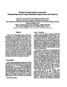
multi-instance tree learners [17], multi-instance rule inducers [17], multi-instance logistic regression methods [18], multi-instance neural networks [19], multi-instance kernel methods [13], multi-instance ensembles [20] and evolutionary algorithms [21]. III. R ELIEF F-MI A LGORITHM This section specifies the filter feature selection algorithm adapted for MIL. First, the main steps of its procedure are detailed. Then, the new definition of distance between bags and the calculation of the difference between attributes are commented on. A. Description of the Method ReliefF-MI is based on the principles of the ReliefF algorithm [3]. This method works by randomly sampling instances from the training data. For each sampled instance R, its k nearest neighbors from the same class (called nearest hit) and the opposite class of each sampled instance (called nearest miss) are found. Multi-class datasets are handled by finding the nearest neighbors from each class that are different from the class of the current sampled instance, and weighting their contributions by the prior probability of each class estimated from the training data. The weight updating of attribute A (W [A]) is computed as the average of all the examples of magnitude of the difference between the distance to the k nearest hits and the distance to the k nearest misses, projecting on the attribute A. Each weight reflects its ability to distinguish among class labels, thus a high weight indicates that there is differentiation to this attribute among instances from different classes and it holds the same value for instances in the same class. Features are ranked by weight and those that exceed a user-specified threshold are selected to form the final subset. In the next section, the calculation of nearest neighbor and the definition of diffbag function applied to bag will be studied. B. Applying the algorithm with multi instance data The ReliefF algorithm estimates the quality of attributes according to how well their values distinguish between the instances that are near to each other. In MIL the distance between two patterns has to be calculated taking into account that each pattern contains one or more instances. The gist of this type of learning is to make a decision based on similarity because each example is a set of instances, so the similarity function needs to be revised since, e.g. the Manhattan distance measure schema is not applicable. The difference between the traditional and MIL cases can be seen in Figure 1. Figure 1(a) shows the calculation in a traditional supervised learning scenario. In this case, the correspondence between a pattern and an instance is one to one and a simple Manhattan distance computing the distance between two corresponding feature vectors can be used. Figure 1(b) shows the case in MIL where the

d(A,B)

A

B

a1

b1

A(a11,a21,…,a1n)

B(b11,b21,…,b1n)

(a) Distance with Single Instances d(A,B)

A

a2

a1 a5

B

b1 a3

a4

a7

a6

b3

b2

b5

b4

X

b6

A(a11,a21,…,a1n) A(a21,a22,…,a2n)

B(b11,b21,…,b1n) B(b21,b22,…,b2n)

. . .

. . .

A(a71,a72,…,a7n)

B(b61,b62,…,b6n)

(b) Distance with Multiple Instances Figure 1.

ing on the class of the pattern, because the information on the examples differs if we evaluate the distance between two positive or negative patterns or between one positive and one negative pattern. Let Ri denote the bag selected in the current iteration. Ri contains three instances (Ri1 , Ri2 , Ri3 ). Let Hj denote the j th bag of the k nearest hit selected in the current iteration. Hj contains four instances, (Hj1 , Hj2 , Hj3 , Hj4 ). Let Mj be the j th bag of the k nearest misses selected in the current iteration. It contains six instances, (Mj1 , Mj2 , Mj3 , Mj4 , Mj5 , Mj6 ). • If both patterns are negative, we can be sure that there is no instance in the pattern that represents the concept that we want to learn. Therefore, an average distance will be used to measure the distance between these bags because all instances are guaranteed to be negative,

Havg (Ri , Hj ) =

•

Differences between Single and Multiple Instance

correspondence between a pattern and an instance is one to many. Therefore, the distance between the two patterns has to take into consideration the distance between two sets of feature vectors with different number of features. Therefore, the Manhattan distance is no longer applicable in this setting. We should also do not forget that labels are known only for bags of instances, but not for the individual instances. If we know that a bag is positive, then we can deduce that at least one of its instances is positive. However, there is no information about how many of them are positive and what instances exactly are positive. In the example in Figure 1(b), the pattern A, the most commonly called bag, has seven different instances and the B bag has six different instances. For example, if A is positive, it might contain four negative instances and three positive ones, but we do not know this information, we know only that at least one of the instances is positive. In the literature, there are different distance-based approaches that have been proposed to solve MI problems [22]. The most extensively used metric is the Hausdorff Distance [23] that measures the distance between two sets. Several adaptations of this measurement have been implemented: maximal Hausdorff distance [23], minimal Hausdorff distance [17] and average Hausdorff distance [22]. We designed a new metric for ReliefF-MI that we called Adapted Hausdorff distance. The reason that has led us to design this new metric is to consider specifically for each distance, the maximum information in this situation. Thus, this metric represents different calculations depend-

r∈Ri

minh∈Hj ||r − h|| +

X

minr∈Ri ||h − r||

h∈Hj

|Ri | + |Hj |

If both patterns are positive, the only real information is that at least one instance in each of them represents the concept that we want to learn, although there is no information about which specific instance or set represents the concept. Therefore, we use minimal distance to measure their distance, Hmin (A, B), because the positive instances have higher probability of being near to each other, Hmin (Ri , Hj ) = minr∈Ri minh∈Hj ||r − h||

•

Finally, if we evaluate the distance between patterns where one of them is a positive bag and the other is a negative one, we take the maximal distance, Hmax (A, B), because the instances in the different classes are probably outliers between the two patterns, Hmax (Ri , Hj ) = max{hmax (Ri , Hj ), hmax (Hj , Ri )} where hmax (Ri , Hj ) = maxr∈Ri minh∈Hj ||r − h||

Besides the defined distance metric, it is also necessary to have the function diffbag that computes the difference between two bags for a given attribute. We define it in a following way: • If Ri is positive and Hj is positive then the two nearest instances are considered for updating the weights, 3

4

diffbag (A, Ri , Hj ) = diffinstance (A, Ri , Hj )

•

where Ri3 and Hj4 are instances satisfying this condition. If Ri is negative and Hj is negative then several instances are taken into account for updating the weights of the features. If we suppose

– d(Ri1 , Hj2 ), d(Ri2 , Hj1 ) and d(Ri3 , Hj4 ) are the minimal distances between each instance r ∈ Ri with respect to instances h ∈ Hj ; and – d(Hj1 , Ri1 ), d(Hj2 , Ri1 ), d(Hj3 , Ri2 ) and d(Hj4 , Ri3 ), are the minimal distances between each instance h ∈ Hj with respect to the instances r ∈ Ri ; then the function diff would be specified as following, 1 diffbag (A, Ri , Hj ) = r+h ∗ [diffinstance (A, Ri1 , Hj2 )+ diffinstance (A, Ri2 , h1j ) + diffinstance (A, Ri3 , h4j )+ diffinstance (A, Hj1 , Ri1 ) + diffinstance (A, Hj2 , Ri1 )+ diffinstance (A, Hj3 , Ri2 ) + diffinstance (A, Hj4 , Ri3 )]

•

Finally, if Ri is positive and Mj is negative or viceversa, one instance from each bag is selected to update the feature weight such that these instances are the farthest between all minimal instances, 1

2

diffbag (A, Ri , Mj ) = diffinstance (A, Ri , Mj )

where Ri3 and Hj4 are instances satisfying this condition. Note that the function diffinstance computes the difference between two particular instances for a given attribute. The total distance is simply the sum of distances throughout all attributes. When dealing with nominal attributes, function diff(A, Ix , Iy ) is defined as: ½ diffinstance (A, Ix , Iy ) =

0; 1;

value(A, Ix ) = value(A, Iy ) otherwise

and for numerical attributes as: diffinstance (A, Ix , Iy ) =

|value(A, Ix ) − value(A, Iy )| max(A) − min(A)

where Ix and Iy two different instance in the data set. It is also used to calculate the distance between instances to find the nearest neighbors. IV. E MPIRICAL S TUDY We compare the performance of seventeen popular MIL algorithms on three benchmark datasets which represent the problem of image categorization. We apply these algorithms on the original datasets with all the features present and on the datasets after the dimensionality reduction. In the following we first consider the application domains and experimental settings and then discuss the obtained results. A. Problem Domains and Experimental Setting All three datasets that we use in our experiment are related to the problem of content-based image categorization where the main task consists of identifying the intended target object(s) in images. From the MIL perspective, this problem can be represented by treating each image as a bag of segments which are modeled as instances. An image

is positive if at least one of the segments contains the object in question, and it is negative otherwise. The detailed information about three data sets is summarized in Table I. To evaluate the performance of the proposed ReliefFMI feature selection method we experiment with different representative paradigms used in MIL to date: methods based on diverse density: MIDD, MIEMDD and MDD; methods based on logistic regression: MILR; methods based on Support Vector Machines: SMO and MISMO which uses the SMO algorithm for SVM learning in conjunction with an MI kernel; distance-based approaches: CitationKNN and MIOptimalBall; methods based on rules: such as PART, Bagging with PART and AdaBoost with PART using MIWrapper and MISimple approach (they are different adaptations for working with MIL); method based on decision tree learning: MIBoost, and methods based on Naive Bayes. More information about these algorithms and their implementation can be found in WEKA [24]. We used 10-fold cross validation procedure to evaluate the generalization performance of the classifiers trained on the original dataset and on different feature subsets. Stratification procedure is used to ensure that each fold contains roughly the same proportions of different classes and the validation method is adapted to MIL to preserve the bag structure composed by different instances. The datasets (including the ranking of features) used in this work will be made available for other researchers at http://www.uco.es/ grupos/kdis/mil/fs. Our feature selection method assigns a real-value weight to each feature to indicate its relevance to the problem. First, the features are ranked according to these weighing, and then a threshold is set to select a subset of important features. To show the influence of the dimensionality reduction on the different MIL classification algorithm, we consider different feature subsets, including the original feature set (i.e. with all the features), and seven other different sets that correspond to the thresholds leaving 10% - 70% of the original features. B. Experimental Results Table II reports on results of accuracy, sensitivity and specificity for the Tiger, Fox and Elephant datasets with different numbers of features. We present the averages from the 10-fold cross validation. Table I G ENERAL I NFORMATION ABOUT THE DATASETS F EATURE Elephant P OSITIVE BAGS N EGATIVE BAGS T OTAL BAGS ATTRIBUTE N UMBER I NSTANCE N UMBER AVERAGE BAG S IZE

100 100 200 230 1391 6.96

DATASET Tiger

Fox

100 100 200 230 1220 6.10

100 100 200 230 1320 6.60

Table II R ESULTS OF ACCURACY USING R ELIEF MI WIHT DIFFERENT NUMBER OF F EATURES A LGORITHMS citationKNN MDD MIBoost (RepTree) MIBoost (DecisionStump) MIDD MIEMDD MIRL MIOptimalBall MISMO (RBF Kernel) MISMO (Polynomial Kernel) MIWrapper (AdaBoost&PART) MIWrapper (Bagging&PART) MIWrapper (PART) MIWrapper (SMO) MIWrapper (Naive Bayes) MISimple (AdaBoost&PART) MISimple (PART)

10% 0.815 0.805 0.855 0.805 0.770 0.770 0.875 0.740 0.855 0.820 0.860 0.865 0.840 0.820 0.820 0.845 0.780

20% 0.830 0.745 0.845 0.805 0.740 0.700 0.780 0.720 0.795 0.815 0.825 0.850 0.820 0.805 0.770 0.835 0.740

30% 0.805 0.745 0.820 0.780 0.740 0.730 0.830 0.665 0.795 0.815 0.840 0.860 0.795 0.805 0.710 0.840 0.780

40% 0.775 0.735 0.840 0.780 0.700 0.740 0.850 0.620 0.800 0.800 0.845 0.830 0.775 0.795 0.730 0.835 0.780

50% 0.775 0.750 0.825 0.780 0.755 0.750 0.850 0.625 0.800 0.785 0.820 0.815 0.790 0.800 0.760 0.805 0.760

60% 0.500 0.735 0.825 0.780 0.750 0.740 0.840 0.625 0.795 0.780 0.790 0.810 0.780 0.800 0.760 0.795 0.765

70% 0.500 0.745 0.825 0.780 0.735 0.745 0.840 0.625 0.795 0.780 0.790 0.810 0.780 0.800 0.760 0.795 0.765

100% 0.500 0.755 0.825 0.780 0.740 0.745 0.840 0.625 0.795 0.785 0.790 0.810 0.780 0.800 0.760 0.795 0.765

A LGORITHMS citationKNN MDD MIBoost (RepTree) MIBoost (DecisionStump) MIDD MIEMDD MILR MIOptimalBall MISMO (RBF Kernel) MISMO (Polynomial Kernel) MIWrapper (AdaBoost&PART) MIWrapper (Bagging&PART) MIWrapper (PART) MIWrapper (SMO) MIWrapper (Naive Bayes) MISimple (AdaBoost&PART) MISimple (PART)

10% 0.615 0.660 0.710 0.700 0.695 0.615 0.635 0.535 0.650 0.655 0.665 0.605 0.620 0.690 0.680 0.650 0.665

20% 0.630 0.680 0.655 0.660 0.660 0.635 0.605 0.540 0.620 0.645 0.675 0.615 0.610 0.685 0.625 0.680 0.660

30% 0.570 0.655 0.685 0.670 0.670 0.660 0.575 0.520 0.600 0.635 0.645 0.605 0.585 0.655 0.600 0.650 0.670

40% 0.605 0.710 0.660 0.655 0.665 0.650 0.545 0.515 0.600 0.605 0.655 0.600 0.540 0.630 0.585 0.615 0.630

50% 0.535 0.685 0.670 0.650 0.665 0.585 0.510 0.530 0.595 0.595 0.685 0.605 0.540 0.635 0.590 0.635 0.635

60% 0.500 0.705 0.670 0.650 0.675 0.640 0.515 0.530 0.595 0.580 0.685 0.605 0.550 0.635 0.590 0.635 0.635

70% 0.500 0.710 0.670 0.650 0.660 0.645 0.515 0.530 0.595 0.585 0.685 0.605 0.550 0.635 0.590 0.635 0.635

100% 0.500 0.700 0.670 0.650 0.655 0.600 0.510 0.530 0.590 0.580 0.685 0.600 0.550 0.635 0.590 0.625 0.635

A LGORITHMS citationKNN MDD MIBoost (RepTree) MIBoost (DecisionStump) MIDD MIEMDD MILR MIOptimalBall MISMO (RBF Kernel) MISMO (Polynomial Kernel) MIWrapper (AdaBoost&PART) MIWrapper (Bagging&PART) MIWrapper (PART) MIWrapper (SMO) MIWrapper (Naive Bayes) MISimple (AdaBoost&PART) MISimple (PART)

10% 0.745 0.705 0.840 0.830 0.755 0.715 0.835 0.775 0.785 0.770 0.840 0.830 0.835 0.705 0.660 0.830 0.775

20% 0.745 0.765 0.855 0.805 0.790 0.735 0.810 0.720 0.785 0.790 0.850 0.835 0.795 0.685 0.745 0.815 0.760

30% 0.755 0.800 0.825 0.815 0.805 0.760 0.815 0.745 0.830 0.785 0.845 0.840 0.780 0.720 0.725 0.805 0.780

40% 0.775 0.770 0.815 0.815 0.820 0.760 0.825 0.740 0.830 0.790 0.860 0.845 0.820 0.710 0.700 0.835 0.780

50% 0.500 0.780 0.815 0.815 0.785 0.765 0.790 0.730 0.800 0.790 0.840 0.845 0.790 0.715 0.680 0.840 0.765

60% 0.500 0.795 0.815 0.815 0.790 0.755 0.790 0.730 0.800 0.790 0.840 0.845 0.790 0.715 0.680 0.840 0.765

70% 0.500 0.785 0.815 0.815 0.805 0.750 0.790 0.730 0.800 0.790 0.840 0.845 0.790 0.715 0.680 0.840 0.765

100% 0.500 0.800 0.815 0.815 0.825 0.730 0.780 0.730 0.800 0.790 0.840 0.845 0.790 0.715 0.680 0.840 0.765

It should be noticed that feature selection may help not only to improve the generalization accuracy but also to learn more compact, easily interpreted representation of the target concept. The algorithms differ in the amount of emphasis they place on feature selection. At one extreme there are algorithms such as the simple nearest neighbor learner that classifies novel examples by retrieving the nearest stored training example, using all available features in its distance computations (such as, CitationKNN and MIOptimaBall). Towards the other extreme there are algorithms that explic-

itly try to focus on relevant features and ignore irrelevant ones. Decision tree inducers are examples of this approach (such as, the MIBoost algorithms with Repetition Tree and Decision Stump). In both cases feature selection prior to learning can be beneficial. Reducing the dimensionality of the data reduces the size of the hypothesis space and allows algorithms to operate faster and more effectively. Also, it has been seen that the methods that are less sensitive to the use of dimensionality reduction are those based on diverse density (such as, MDD, MIDD, MIEMDD). To determine the advantages of applying this features

Percentage of Features 10% Features 20% Features 30% Features 40% Features 50% Features 60% Features 70% Features 100% Features

Accuracy Ranking 2.863 4.069 3.814 4.588 4.843 5.167 5.167 5.490

Table IV F RIEDMAN T EST

χ2 (α = 0.95) 12.020

Value Test 45.327

Conclusion Reject null hypothesis

selection method, we performed a statistical test determining whether there are statistically significant differences in the performance results when algorithms use data sets with different number of features. We chose Friedman test – a non parametric test that compares the average ranks of the considered algorithms. These ranks show which algorithm obtains the best results. Note that the percentage of features with a value closest to 1 indicates that the algorithms considered in this study generally obtain better results using that percentage of features than other percentages of features. The ranks obtained by each feature set can be seen in Table III where the lowest rank values are obtained when algorithms use a set with a reduced number of features. Thus, the best accuracy values are obtained by algorithms when they use the data set with lower number of features (that is, 10% of features). If the number of features is increased the accuracy values obtained by algorithms become worse and therefore the rank of these dataset has a higher value. In Table IV, the Friedman test results indicate that there are statistically significant differences in the results when using different number of features. We perform a posthoc test, namely the Bonferroni-Dunn test [25], to find the significant differences that occur when different percentages of features were used. Figure 2 shows the application of this test which determines a threshold and any algorithm with a higher rank value than that threshold is considered to be worse than the control algorithm (in this case, the best option is to use of 10% of the most relevant features with a value rank of 2.863 and the threshold set to 4.186). Thus, the use of a higher percentage of 30% produces that algorithms results in worse performance. In general, we can conclude that the use of Relief-MI improves the performance of the considered MIL algorithms. Using 100% of features results in the worst performance for

all algorithms and on all datasets (this threshold corresponds to the highest rank value). Using 10%, 20% and 30% of the most relevant features always result in better performance. V. R ELATED WORK The problem of feature selection in MIL setting has not been studied extensively yet. To the best of our knowledge, no filter approach for feature selection that utilizes the labels of bags has been proposed so far. Existing approaches fall either in the wrapper category, i.e. different feature subsets are evaluated based on the performance of a MIL classifier learnt from the data presented by these subsets, or the embedded category, i.e. feature selection is designed as part of a MIL algorithm. The most well-known feature selection approaches for MIL include: feature scaling with Diverse Density and principal component analysis for BP-MIP MIL algorithm presented in [26], MI-AdaBoost [27] and hyperclique pattern mining [6] where region-based image retrieval is formulated as a MIL problem, and Bayesian MIL algorithm that uses feature selection [28]. Although these approaches have shown promising results in terms of accuracy improvement, they still have two main limitations. Namely, they are biased for particular MIL classifiers, and what is more important, they are not efficient for truly high-dimensional problems, because the learning algorithm has to be called on repeatedly for the evaluation of every considered feature subset (and the search space can be quite large even if a heuristic search is employed). In contrast, the filter approach that we propose in this paper is applicable for high dimensional dataset and has a more generic nature that is it operates independently of MIL algorithm to be applied on the datset with the reduced dimensionality. VI. C ONCLUSIONS The task of identifying the most important attributes and performing dimensionality reduction by discarding the 6

5

Ranking

Table III A LGORITHM R ANKING U SING D IFFERENT P ERCENTAGE OF F EATURES

4

3

2

10%

20%

30% 40% 50%

60%

70% 100%

Features Used

Figure 2.

Bonferroni Dunn Test (p < 0.05)

irrelevant and redundant attributes is known to be of prior importance in supervised learning. Many features selection approaches have been introduced to accomplish this task. Filter-based approaches, which are known to be most efficient and reasonably effective for the traditional settings, are not directly applicable for finding the most important features in multiple instance learning. This situation calls for the development of new or an adaptation of existing approaches for the settings when only the labels for bags of instances, but not for the individual instances, are known in the training data. In this paper we considered ReliefF-MI algorithm based on ReliefF principles. ReliefF-MI can be applied to continuous and discrete problems. It is expected to be faster than the existing wrapper methods for feature selection and can be applied to any of the existing MIL algorithms, since feature selection is performed as the preprocessing step. Experimental results showed the effectiveness of our approach for seventeen MIL algorithms in three different benchmark applications. We hope that these promising results will promote the development of other filter approaches for feature selection in MIL. ACKNOWLEDGMENT The authors gratefully acknowledge the financial support provided by the Spanish department of Research under TIN2008- 06681-C06-03, P08-TIC-3720 Projects and FEDER funds.

[7] H. T. Pao, S. C. Chuang, Y. Y. Xu, and H. . Fu, “An EM based multiple instance learning method for image classification,” Expert Systems with Applications, vol. 35, no. 3, pp. 1468– 1472, 2008. [8] X. Qi and Y. Han, “Incorporating multiple SVMs for automatic image annotation,” Pattern Recognition, vol. 40, no. 2, pp. 728–741, 2007. [9] T. G. Dietterich, R. H. Lathrop, and T. Lozano-Perez, “Solving the multiple instance problem with axis-parallel rectangles,” Artifical Intelligence, vol. 89, no. 1-2, pp. 31–71., 1997. [10] O. Maron and T. Lozano-P´erez, “A framework for multipleinstance learning,” in NIPS’97: Proceedings of Neural Information Processing System 10, Denver, Colorado, USA, 1997, pp. 570–576. [11] A. Zafra, S. Ventura, C. Romero, and E. Herrera-Viedma, “Multi-instance genetic programming for web index recommendation,” Expert System with Applications, vol. 36, pp. 11 470–11 479, 2009. [12] X. Chen, C. Zhang, S. . Chen, and S. Rubin, “A humancentered multiple instance learning framework for semantic video retrieval,” IEEE Transactions on Systems, Man and Cybernetics Part C: Applications and Reviews, vol. 39, no. 2, pp. 228–233, 2009.

R EFERENCES

[13] Z. Gu, T. Mei, J. Tang, X. Wu, and X. Hua, “MILC2: A multi-layer multi-instance learning approach to video concept detection,” in MMM’08: Proceedings of the 14th International Conference of Multimedia Modeling, Kyoto, Japan, 2008, pp. 24–34.

[1] A. Zafra, M. Pechenizkiy, and S. Ventura, “Reducing dimensionality in multiple instance learning with a filter method,” in HAIS (2), ser. Lecture Notes in Computer Science, E. Corchado, M. G. Romay, and A. Savio, Eds., vol. 6077. Springer, 2010, pp. 35–44.

[14] A. Zafra and S. Ventura, “Predicting student grades in learning management systems with multiple instance genetic programming,” in EDM’09: Proceedings of the 2sd Conference on Educational Data Mining, Cordoba, Spain, 2009, pp. 309– 319.

[2] K. Kira and L. Rendell, “A practical approach to feature selection,” in ICML’92: Proceedings of the 9th International Conference in Machine Learning, 1992, pp. 249–256. [3] I. Kononenko, “Estimating attributes: analysis and extension of relief,” in ECML’94: Proceedings of the 7th European Conference in Machine Learning. Springer-Verlag, 1994, pp. 171–182. [4] S. Robnik and I. Kononenko, “An adaptation of relief for attribute estimation in regression,” in ICML’94: Proceedings of the 14th International Conference on Machine Learning. Morgan Kaufmann, 1997, pp. 296–304.

[15] Q. Zhang and S. Goldman, “EM-DD: An improved multipleinstance learning technique,” in NIPS’01: Proceedings of Neural Information Processing System 14, Vancouver, Canada, 2001, pp. 1073–1080. [16] J. Wang and J.-D. Zucker, “Solving the multiple-instance problem: A lazy learning approach,” in ICML’00: Proceedings of the 17th International Conference on Machine Learning, Standord, CA, USA, 2000, pp. 1119–1126.

[5] S. Andrews, I. Tsochantaridis, and T. Hofmann, “Support vector machines for multiple-instance learning,” in NIPS’02: Proceedings of Neural Information Processing System, Vancouver, Canada, 2002, pp. 561–568.

[17] Y.-Z. Chevaleyre and J.-D. Zucker, “Solving multiple-instance and multiple-part learning problems with decision trees and decision rules. Application to the mutagenesis problem,” in AI’01: Proceedings of the 14th of the Canadian Society for Computational Studies of Intelligence, LNCS, vol. 2056, Ottawa, Canada, 2001, pp. 204–214.

[6] G. Herman, G. Ye, J. Xu, and B. Zhang, “Region-based image categorization with reduced feature set,” in Proceedings of the 10th IEEE Workshop on Multimedia Signal Processing, Cairns, Qld, 2008, pp. 586–591.

[18] X. Xu and E. Frank, “Logistic regression and boosting for labeled bags of instances,” in PAKDD’04: Proceedings of the 8th Conference of Pacific-Asia. LNCS, vol. 3056, Sydney, Australia, 2004, pp. 272–281.

[19] Y.-M. Chai and Z.-W. Yang, “A multi-instance learning algorithm based on normalized radial basis function network,” in ISSN’07: Proceedings of the 4th International Symposium on Neural Networks. LNCS, vol. 4491, Nanjing, China, 2007, pp. 1162–1172. [20] Z.-H. Zhou and M.-L. Zhang, “Solving multi-instance problems with classifier ensemble based on constructive clustering,” Knowledge and Information Systems, vol. 11, no. 2, pp. 155–170, 2007. [21] A. Zafra, E. Gibaja, and S. Ventura, “Multi-instance learning with multi-objective genetic programming for web mining,” Applied Soft Computing. In Press, 2009. [22] M.-L. Zhang and Z.-H. Zhou, “Multi-instance clustering with applications to multi-instance prediction,” Applied Intelligence, vol. 31, pp. 47–68, 2009. [23] G. Edgar, Measure, topology, and fractal geometry. Third Edition. Springer-Verlag, 1995. [24] I. H. Witten and E. Frank, Data Mining: Practical Machine Learning Tools and Techniques. Second Edition. Morgan Kaufmann, 2005. [25] O. J. Dunn, “Multiple comparisons among means,” Journal of the American Statistical Association, vol. 56, no. 293, pp. 52–64., 1961. [26] M.-L. Zhang and Z.-H. Zhou, “Improve multi-instance neural networks through feature selection,” Neural Processing Letter, vol. 19, no. 1, pp. 1–10, 2004. [27] X. Yuan, X.-S. Hua, M. Wang, G.-J. Qi, and X.-Q. Wu, “A novel multiple instance learning approach for image retrieval based on adaboost feature selection,” in ICME’07: Proceedings of the IEEE International Conference on Multimedia and Expo. Beijing, China: IEEE, 2007, pp. 1491–1494. [28] V. C. Raykar, B. Krishnapuram, J. Bi, M. Dundar, and R. B. Rao, “Bayesian multiple instance learning: automatic feature selection and inductive transfer,” in ICML ’08: Proceedings of the 25th international conference on Machine learning. New York, USA: ACM, 2008, pp. 808–815.