[2] E. Domany, D. Mukamel, B. Nienhuis and A. Schwimmer, Nucl. Phys. ... F. David, P. Ginsparg and J. Zinn-Justin, (Elsevier: Les Houches session LXII, 1994).
arXiv:cond-mat/9903242v1 [cond-mat.stat-mech] 16 Mar 1999
Finite average lengths in critical loop models Jesper Lykke Jacobsen and Jean Vannimenus Laboratoire de Physique Statistique1 , Ecole Normale Sup´erieure, 24 rue Lhomond, F-75231 Paris Cedex 05, France.
ABSTRACT A relation between the average length of loops and their free energy is obtained for a variety of O(n)-type models on two-dimensional lattices, by extending to finite temperatures a calculation due to Kast. We show that the (number) averaged loop length L stays finite for all non-zero fugacities n, and in particular it does not diverge upon entering the critical regime (n → 2+ ). Fully packed loop (FPL) models with n = 2 seem to obey the simple relation L = 3Lmin , where Lmin is the smallest loop length allowed by the underlying lattice. We demonstrate this analytically for the FPL model on the honeycomb lattice and for the 4-state Potts model on the square lattice, and based on numerical estimates obtained from a transfer matrix method we conjecture that this is also true for the two-flavour FPL model on the square lattice. We present in addition numerical results for the average loop length on the three critical branches (compact, dense and dilute) of the O(n) model on the honeycomb lattice, and discuss the limit n → 0. Contact is made with the predictions for the distribution of loop lengths obtained by conformal invariance methods.
PACS numbers: 05.50.+q, 64.60.-i, 75.10.Hk
1
Laboratoire associ´e aux universit´es Paris 6, Paris 7 et au CNRS.
1
Introduction
Loop models appear in various contexts in statistical physics, not only as models of various phases of polymers [1] but also in the high-temperature expansion of the O(n) spin model [2, 3], in surface growth models [4], in efficient cluster-flipping Monte Carlo methods [5], and in the study of quantum spin systems [6]. They have deep connections with other well-studied statistical models, such as the eight-vertex, colouring and Potts models [7, 8], and they can be viewed as toy models for the study of string theories. One of their main interests is that they provide examples of systems involving extended degrees of freedom, rather than local ones as in spin systems, for which many exact results have been obtained in d = 2 using Bethe ansatz [7], Coulomb gas [9] and conformal invariance methods [10]. The basic O(n) loop model is defined through the partition function Z(n, t) =
X
nP tV ,
(1.1)
C
where n is the loop fugacity, which controls the number P of different loops (“paths”) in the configuration C, and t is a temperature-like variable which controls the number V of empty sites (“voids”) not covered by any loop, the total number of sites on the lattice being N.2 For non-crossing loops on the honeycomb and square lattices a phase transition occurs at n = nc = 2, for all temperatures below a lattice-dependent tc [3, 11]. That transition is very weak and is reminiscent of the Kosterlitz-Thouless transition for the XY spin model, as the free energy only has an essential singularity. The geometrical interpretation is simple: For n > nc the configurations contributing to Z only contain finite loops in the thermodynamic limit, whilst for n ≤ nc there appear “infinite” loops whose extent diverges with the lattice size. This is analogous to what happens in lattice percolation models, where an infinite cluster appears when the site (or bond) occupation probability is above a threshold value pc [12], and indeed the perimeters of percolation clusters can be viewed as special cases of loops [10, 13]. 2
This is the standard definition of the O(n) model on the honeycomb latttice [3]. On lattices with
higher coordination number a given site may be visited by more than one loop, necessitating the introduction of further weights in Eq. (1.1) [11]. We shall come back to this point later on.
1
Explicit formulae for the free energy per site, defined as 1 log Z(n, t), N →∞ N
F (n, t) = lim
(1.2)
can be obtained [14, 15, 16] along certain critical lines in the (n, t) plane [3] for the honeycomb lattice, but the distribution of loop lengths cannot be inferred from the partition function, and information about it is obtained numerically [8] or through scaling and conformal invariance methods [17] (see the lectures by Cardy [10] for an introduction to the geometric properties of loop models). We show in the first part of the present work that a simple relation, first derived by Kast at t = 0 in the honeycomb O(n) model [18], can be generalised to finite temperatures and to a variety of other loop models. It gives the average loop length L from the knowledge of the free energy and its derivatives with respect to n and t only. In the second part we use the exactly known results for F (n, t = 0) to calculate analytically that average length at the fugacity where a transition occurs, nc = 2. We present next very accurate numerical calculations of the average loop length, using a transfer matrix method and our relation, at finite temperatures and for the zero-temperature O(n) model on the square lattice. For both the t = 0 (fully packed) model on the honeycomb lattice and for the 4-state Potts model on the square lattice we find the exact result L = 3Lmin ,
(1.3)
where Lmin is the minimal loop length allowed by the given lattice. Contrary to what was suggested in Ref. [18] on the basis of numerical results, the average length thus remains finite for n = nc , and indeed for all non-zero n. This is a priori counter-intuitive, as one would naively expect the appearance of infinite loops below nc to be reflected in a diverging average length, but we show in the last part of the paper that this result is not in contradiction with the predictions of conformal invariance.
2
Average loop length and the free energy
The average length of non-crossing loops in a given configuration C on the honeycomb lattice is given by hL(C)i = 2
N −V , P
(2.1)
since a given site belongs to at most one loop, and its ensemble average with respect to Eq. (1.1) is L=
1 XN −V P V n t . Z C P
(2.2)
Introducing the partial derivatives ∂n and ∂t with respect to n and t one has: ∂n (ZL) = ∂t Z =
1X (N − V )nP tV , n C
(2.3)
1X V nP tV . t C
(2.4)
Eliminating the average number of voids between these two relations gives ∂n (ZL) =
1 [NZ − t ∂t Z] , n
(2.5)
or, in terms of the free energy, ∂n L 1 + L ∂n F = [1 − t ∂t F ] . N n
(2.6)
Now, if ∂n L remains finite the first term on the left-hand side of Eq. (2.6) becomes negligible in the thermodynamic limit, and we obtain a simple relation between L and the partial derivatives of F (n, t), L=
1 − t ∂t F , n ∂n F
(2.7)
which generalizes Kast’s relation [18] to non-zero temperature. Several remarks are in order here: • The validity of relation (2.7) relies on the finiteness of ∂n L, which in turn, as is seen from Eq. (2.7), holds as long as ∂n ∂t F and ∂n2 F remain finite, and n and ∂n F
do not vanish. As we shall see below, these conditions can be shown explicitly to be fulfilled for fully packed (t = 0) loops on the honeycomb lattice, for all n > 0. • The knowledge of F (n, t) along a critical line in the (n, t) plane is not sufficient to obtain the average length L, as it provides only one relation between ∂n F and ∂t F , through the total derivative dn F , and in general it is not possible to express L as a function of dn F alone.
3
• One can also write relations for P , the ensemble average number of loops [10]: P =
1X P (C)nP tV . Z C
(2.8)
n ∂n Z = Nn ∂n F. Z
(2.9)
One has from Eqs. (1.1) and (1.2) P =
Taking now the derivative of Eq. (2.9) with respect to n, one finds
∂n Z ∂2 Z ∂n Z ∂n P = + n n − Z Z Z
!2
=
� 1� 2 2 P −P , n
(2.10)
which yields an explicit expression for the fluctuations in the loop number: � 1 � 2 2 P − P = n ∂n F + n2 ∂n2 F. N
(2.11)
Relations (2.9) and (2.11) show that the average number of loops is extensive (except for n = 0) and that its fluctuations become negligible in the thermodynamic limit, as long as ∂n F and ∂n2 F remain finite. It is also interesting to note that for a perfect gas at fixed chemical potential the fluctuations in the number M of particles in a given volume are given by 2
M 2 − M = M,
(2.12)
so the second term on the right-hand side of Eq. (2.11) may be viewed as a correction with respect to the fluctuations in a “perfect gas” of loops, induced by the nonoverlapping condition. Before leaving this Section we briefly comment on the appropriate form of the relation (2.7) for lattices with higher coordination number. As an example, consider the O(n) model on the square lattice, for which the partition function has a slightly more complicated form than the one given in Eq. (1.1), since each vertex can be visited by the loops in several ways that are unrelated by rotational symmetry. Following Ref. [11] we define ZO(n) =
X
tNt uNu v Nv w Nw nP ,
C
4
(2.13)
where Nt , Nu , Nv and Nw are the number of vertices visited by respectively zero, one turning, one straight, and two mutually avoiding loop segments. The relation (2.1) must be replaced by hL(C)i =
N − Nt + Nw , P
(2.14)
and under assumptions on the higher derivatives identical to those given above the generalisation of Eq. (2.7) finally reads L ∂n F =
3
1 (1 − t ∂t F + w ∂w F ) . n
(2.15)
Zero-temperature case: Fully packed loops
At t = 0 configurations containing voids do not contribute to Z, and on the honeycomb lattice every site must belong to one and only one loop. The system of loops is then called fully packed or “compact”, to distinguish it from the “dense” phase [3, 17] with a finite density of voids found at non-zero t. A necessary condition for the t = 0 line to be stable (in the RG sense) is that Z(n, t) is invariant under the replacement of t by −t
[19].3 This symmetry criterion is fulfilled because the honeycomb lattice is bipartite and
hence only allows for loops of even length. For the model at hand the condition is also sufficient (see Ref. [20] for an example where this is not the case), and as a consequence, the t = 0 line is critical for n ≤ 2 and fully packed loops are in a different universality class than dense loops [19, 21, 22, 23, 24]. The relation (2.7) reduces for t = 0 to the form obtained by Kast [18]: L(n) =
1 , nF0′ (n)
(3.1)
where F0 (n) = F (n, t = 0), and it is particularly interesting as explicit expressions are known for the free energy in that case, thanks to the work of Baxter [25], Reshetikhin [26], Batchelor et al. [21], and Kast himself [18]. One has for the free energy per site of the honeycomb lattice • for n < 2: F0 (n) =
1 2
Z
∞
dx
−∞
sinh2 λx sinh(π − λ)x , x sinh πx sinh 3λx
where λ > 0 and n = 2 cos λ. 3
Negative values of t correspond to an antiferromagnetic interaction in the spin language.
5
(3.2)
• for n > 2:
∞ Y (1 − q −6m+2 )2 1 , F0 (n) = log q 1/3 −6m+4 )(1 − q −6m ) 2 m=1 (1 − q
#
"
(3.3)
where q = eγ and n = 2 cosh γ.
Analytically it is known that at the critical point nc = 2, F0 (n) takes the value [25, 21]4 F0 (2) =
Z
∞
0
∞ 1 1 X du sinh2 u −u log 1 − e =− u sinh 3u 2 m=1 (3m − 1)2
"
#
1 3Γ3 (1/3) = = 0.18956 · · · . log 2 4π 2 #
"
(3.4)
The analytic calculation can be pushed further, noting that for n < 2 Eq. (3.2) can be reexpressed as F0 (λ) − F0 (λ = 0) =
Z
∞
1 sinh3 u 1− du u sinh 3u tanh(πu/λ)
Z
∞
0
= −
"
0
#
dv sinh3 (λv/π) 1 −1 . v sinh(3λv/π) tanh v �
�
(3.5)
This expression can then be expanded in powers of λ. To lowest order this reads: F0 (λ) − F0 (λ = 0) ≃ −
λ2 3π 2
Z
0
∞
dv v
2λ2 e−v =− 2 sinh v 3π
Z
∞
dv
0
λ2 v = − . e2v − 1 36
(3.6)
In terms of the loop fugacity n, this yields
dF0 dF0 dλ 1 = = , dn n→2− dλ dn λ→0+ 36
(3.7)
so we obtain an unexpectedly simple result for the average length of the fully packed loops at the critical point L0 (n = 2) = 18.
(3.8)
A similar analysis can be performed for n > 2, rewriting for example Eq. (3.3) as F0 (n) − F0 (2) =
∞ γ 1 X fm , − 6 2 m=1
(3.9)
with "
4
g(6mγ)g([6m − 4]γ) fm = log g 2 ([6m − 2]γ)
Note that there is a misprint in Eq. (7) of Ref. [21].
6
#
(3.10)
and g(x) = x1 (1 − e−x ). The terms in Eq. (3.9) have been grouped so as to make it more convenient to use the Taylor-McLaurin summation formula ∞ X
fm =
m=1
Z
0
∞
1 1 1 ′′′ dy f (y) − f (0) − f ′ (0) + f (0) + · · · . 2 12 720
(3.11)
The evaluation of Eq. (3.9) for small γ then yields for dF0 /dn|n→2+ the same value as Eq. (3.7). The calculation of d2 F0 /dn2 proceeds along similar lines, and the end result reads d2 F0 1 = for n = 2, dn2 1080
(3.12)
the same value being obtained on both sides of the transition (more generally, one expects all derivatives of F0 (n) to be continuous for n = 2). As λ = 0 (n = 2) is the only point where Eq. (3.2) may have a singularity, we conclude that Kast’s relation (2.7) remains valid in the whole region n < 2, which was not a priori obvious from his derivation. As a by-product one also obtains from Eqs. (2.9) and (2.11) the average number of fully packed loops for n = 2:
P0
n=2
and its fluctuations: P02
− P0
2
n=2
=
N 18
1 1 =N + 18 270 �
(3.13)
�
(3.14)
Another interesting case is the limit of n → 0. This is the compact polymer (Hamiltonian cycle) limit, when a single loop covers all the lattice sites (with adequate boundary conditions). The derivative of Eq. (3.2) can now be evaluated directly:
Thus
dF0 4 = dλ λ=π/2 π
Z
0
∞
du
1 − cosh 2u 1 2 = − √ . 2 (1 + 2 cosh 2u) π 3 3
dF0 dλ 1 dF0 1 , = = √ − dn n=0 dλ dn λ=π/2 3 3 2π
(3.15)
(3.16)
and invoking once again Eq. (3.1) the average loop length L0 (n) diverges as L0 (n) =
30.0344 · · · + O(1). n
One can also show that the second derivative F ′′ (0) = −0.00684676 · · · is finite. 7
(3.17)
4
Numerical results on the honeycomb lattice
4.1
Zero temperature
We have checked numerically the analytical expressions given in the literature for the free energy of the O(n) model at t = 0, using a previously developed transfer matrix method [19] to compute the partition function for strips of finite width, up to Wmax = 15. The results can be further analysed by exploiting that the dominant finite-size corrections are known from conformal invariance arguments [27, 28] F0 (W ) = F0 (∞) −
πc(n) + ···, 6W 2
(4.1)
where c(n) is the central charge of the model. The latter has been inferred from the Bethe ansatz solution of the model [21] c(n) = 2 −
6e2 with n = 2 cos(πe). 1−e
(4.2)
Carrying out the numerical differentiation on F0 (∞) obtained from Eq. (4.1), rather than on the F0 (W ) which are related to the leading eigenvalue of the transfer matrix spectra, we were able to obtain sufficient accuracy to calculate the derivative dF0 /dn, and hence L0 (n), using formula (2.7). In Fig. 1 we plot L0 (n) in units of Lmin = 6, which is the shortest possible loop length on the honeycomb lattice. To emphasize the fact that the average loop length does not exhibit any singularity at nc = 2 these data are shown without the central charge correction. We point out that it would not have been possible to produce this plot by a direct numerical differentiation of the analytic results, Eqs. (3.2) and (3.3), as these expressions in their present form converge extremely slowly close to the critical fugacity nc = 2. Actually we suspect that it was these difficulties that led Kast [18] to the erroneous conjecture that L(n → 2+ ) diverges. Turning now on the correction (4.1) we find the finite-size values of F0′ (n) given in Table 1. Results are only shown for W a multiple of three, since otherwise the equivalent interfacial representation [22] will be subject to height defects, leading to the introduction of non-trivial twist-like operators in the continuum theory [23]. An extrapolation to the thermodynamic limit W → ∞ can be performed by fitting the residual size dependence 8
Figure 1: Average loop lengths, measured in units of six, for the FPL model on the honeycomb lattice. The finite-size estimates converge rapidly towards the exact value L(n = 2) = 18.
W
F0′ (n = 0)
6 0.03192052 9 0.03304791 12 0.03321945 15 0.03326456 ∞ 0.033296 (3) Eq. (3.16) 0.0332951 · · · Table 1: Finite-size estimates of F0′ (n = 0), corrected for the known value of c, as a function of strip width W . The extrapolated value is found by fitting the residual sizedependence to a 1/W 4 term.
9
to a 1/W 4 term [23]. The result is 1 = 30.034(3), = 0)
F0′ (n
(4.3)
in excellent agreement with the analytical result (3.17). In the same manner we find for n = nc that 1 = 35.96(3), = 2)
F0′ (n
(4.4)
confirming Eq. (3.7). We have also evaluated numerically F0′′ (n = 0) = −0.00686(2), whereas an attempt to compute F0′′ (n = 2) did not lead to a sufficiently accurate result to permit a comparison with Eq. (3.12). The reason for this is a combination of the logarithmic corrections to the scaling form (4.1) [29] and the singularity arising in Eq. (4.2) when taking the second derivative with respect to n at n = nc .
4.2
Non-zero temperature: Dense and dilute loops
As discussed earlier, explicit expressions for F (n, t) are known only along two other special critical lines in the (n, t) plane, for which Bethe ansatz solutions were given in Ref. [14, 15, 16]. These lines, or branches, are given by the relation [3] t2 = 2 ±
√ 2 − n,
(4.5)
where the upper sign corresponds to the “dilute” branch and the lower sign to the “dense” branch. We have already remarked that this knowledge is not sufficient to obtain analytically the average loop length from Eq. (2.7). However, an accurate numerical determination of the partial derivatives ∂n F and ∂t F t is possible, using the same transfer matrix approach as for t = 0 so the variation of L along these lines can be studied in detail. The central charge values used in the extrapolation procedure are now c(n) = 1 −
6e2 with n = 2 cos(πe). 1∓e
(4.6)
The resulting values of L(n) are displayed in Fig. 2. Only the data for strip width W = 9 are displayed, since employing the correction (4.6) renders the residual finite-size effects indistinguishable on the figure. Extrapolating to W = ∞ we obtain for n = nc = 2 L(nc , tc =
√
2) = 19.417(1), 10
(4.7)
Figure 2: Average lengths of dense and dilute loops on the honeycomb lattice, measured in units of six. which is slightly larger than the corresponding value at t = 0. The same is true for the asymptotic n → 0 behaviour on the dense branch, for which the numeric result is Ldense (n) =
35.70(2) + O(1). n
(4.8)
At first sight this finding may seem odd, since the geometrical scaling dimension e2 1 x2 = (1 − e) − 2 2(1 − e)
(4.9)
coincides for the dense and the compact branch [9, 21], implying that the asymptotic distributions of large loops are identical in the two models [17]. However the dense phase has fewer short loops than the compact one, since it is always energetically favourable to trade a length-six loop for some empty space: √ t6 (2 − 2 − n)3 = ≥ 1 (identity at n = 1). n n
(4.10)
Since a length-six loop necessarily has a fixed shape of its perimeter there is no extensive entropy involved in the argument, and our simple energetical consideration suffices. Another remark pertains to the fact that L(n) is an increasing function of n on the dilute branch (and in particular it does not diverge as n → 0). This has a quite elementary explanation in terms of x2 to which we shall come back in Section 6. 11
5
Loops on the square lattice
Many results have also been obtained for systems of loops on the square lattice [7, 8, 11, 23, 24, 30, 31, 32, 33, 34], but now there are several possible definitions of the models, depending on whether one allows the non-overlapping loops to cross at the vertices or not, if there is only one kind of loops or two, and exactly how the loop segments are allowed to turn at the vertices. Following Refs. [23, 24], we consider a model with two kinds (“flavours”) of loops, with respective fugacities n1 and n2 , which both cover all N vertices of the square lattice and can intersect but not overlap. This can be considered as a particular zero-temperature limit [34] of the O(n) model on the square lattice [11]. The partition function and the free energy are given by Z0 (n1 , n2 ) =
X
nP1 1 nP2 2 ,
(5.1)
C
F0 (n1 , n2 ) =
1 log Z0 (n1 , n2 ), N →∞ N lim
(5.2)
where the summation is performed over all doubly compact configurations. The constraint that both types of loops cover all N sites implies that for each configuration the average length of type-1 loops is just hL1 (C)i = N/P1 , and its ensemble average is given by L1 =
1 X N P1 P2 n n . Z 0 C P1 1 2
(5.3)
Repeating the calculation of Section 2 one obtains ∂n1 (Z0 L1 ) = N
Z0 n1
(5.4)
and 1 1 ∂n1 L1 + L1 ∂n1 F0 = . N n1
(5.5)
Now, if ∂n1 L1 remains finite, the first term in the left-hand side of Eq. (5.5) is negligible in the thermodynamic limit, and we obtain L1 =
1 . n1 ∂n1 F0
(5.6)
A similar relation holds for the average length L2 of the second kind of loops, with n2 replacing n1 , and when n1 = n2 both reduce to Kast’s relation (3.1).
12
One can also define the average length L of any loop, regardless of flavour. Following the above line of reasoning this is easily shown to fulfill the relation L=2
L1 L2 . L1 + L2
(5.7)
For n1 = n2 the above statement is trivial. Taking however the limit L2 → ∞ we obtain the curious result that L = 2L1 for n2 → 0,
(5.8)
regardless of the value of n1 . Since the model (5.1) has as yet defied a Bethe ansatz solution, no analytical expressions for F0 (n1 , n2 ) are available (apart from the conjecture F0 (0, 0) =
1 2
log 2 [23]). We
have therefore studied numerically the relation (5.6) as a function of n1 , for different values of n2 = 0, 1 and 2. Transfer matrix computations were performed for strips of even width, up to Wmax = 12, exploiting that [23] c(n1 , n2 ) = 3 −
6e21 6e22 − . 1 − e1 1 − e2
(5.9)
Extrapolating as usual to W = ∞ we find for the average loop lengths at n1 = 2: L1 (n1 = 2, n2 ) =
and for its divergence when n1 → 0:
15.74(5) for n2 = 0 13.95(3) for n2 = 1
(5.10)
11.99(2) for n2 = 2
A = 21.97(6) for n2 = 0 A + O(1) with A = 20.35(3) for n2 = 1 . L1 (n1 → 0, n2 ) = n1 A = 18.96(3) for n2 = 2
(5.11)
A striking fact is that for the symmetric case n1 = n2 = nc = 2, which corresponds to the four-colouring model introduced in Ref. [8], the numerical value of the average length of either kind of loops is Lc /Lmin = 2.997(4),
(5.12)
where we have normalised with respect to the length of the shortest possible loop on the square lattice, Lmin = 4. The ratio (5.12) is extremely close to 3, which by Eq. (3.8) is the exact result for the zero-temperature O(n) model on the honeycomb lattice. 13
In order to see if this could be more than a coincidence, we have looked at another model on the square lattice, describing the q-state Potts model at its selfdual point [7]. We briefly recall how the Potts model is transformed into a loop model [7]: In a first step the spin model (with coupling constant K) is turned into a random cluster model [35]. Each state is now a bond percolation graph in which each connected cluster is weighed by q and each coloured bond carries a factor of (eK − 1). Next, the clusters are traded for loops on the medial graph (the lattice formed by the mid-points of the bonds on the √ original lattice). By the Euler relation each closed loop is weighed by q, and the bond √ weights are (eK − 1)/ q [7]. At the selfdual point the latter equals one by duality, and the exact correspondence is ZPotts = q N/2
X√ C
q P ≡ q N/2 ZLoop ,
(5.13)
where N is the number of sites of the original lattice. Defining F as the free energy per medial site with respect to ZLoop , one has [7] • for n < 2:
1 2
F (n) = where λ > 0 and n =
√
√
∞
−∞
dx
sinh λx sinh(π − λ)x , x sinh πx cosh λx
(5.14)
q = 2 cos λ.
• for n > 2: where n =
Z
∞ e−mλ λ X tanh mλ, F (n) = + 2 m=1 m
(5.15)
q = 2 cosh λ.
The value at the critical point nc = 2 is also known: F (n = 2) =
Z
0
∞
du tanh u e−u = 0.78318 · · · , u
(5.16)
and as in Section 3 we can evaluate the derivative dF/dn|n→2− by examining the difference F (λ) − F (λ = 0) = −
Z
0
∞
dv 1 sinh(λv/π) tanh(λv/π) −1 . v tanh v �
�
(5.17)
At the bottom line we obtain L(n = 2) = 12, 14
(5.18)
or Lc /Lmin = 3, the same result being found also for n → 2+ . For n → 0 the average loop length diverges as L(n) =
16 + O(1). n
(5.19)
Both these results are in excellent agreement with numerical estimates produced by the transfer matrices described in Ref. [36]. Our computations for the Potts model suggest that the result (1.3) is not a mere coincidence, and we feel confident in conjecturing that L/Lmin = 3 is also exactly true for the four-colouring model, cf. Eq. (5.12). It would be quite surprising if this ratio were a new universal quantity, like for instance the ratio of the average loop area to the average square gyration radius, calculated by Cardy [10]. Rather it is reminiscent of the “quasiinvariants” found in percolation theory: For a large variety of lattices, the percolation thresholds are observed to be little lattice-dependent, for a fixed dimensionality, once they are properly normalised taking into account the coordination number [37].
6
Discussion and contact with conformal invariance predictions
The most striking aspect of the results presented above is that the average loop length remains finite, even inside the critical phase where the correlation length, which is roughly the size of the largest loop in a typical configuration, diverges. In fact, a little thought shows that the apparent paradox comes from the definition of “average length”: In our calculations all loops are equally weighted, irrespective of their length. This is called the “number average” in polymer theory, to distinguish it from the “weight average”, where each polymer contributes with a weight proportional to its length. Depending on the quantity being measured, these and still other averages are relevant in order to compare theoretical predictions with experiments (see, e.g., the treatise by des Cloizeaux and Jannink [38] for a detailed discussion). An analogous situation arises in percolation theory, when one defines the “average cluster size” [12]: If one means “the average size of the cluster on which an ‘ant’ lands at random”, the weight average has to be taken, which is different from the average size obtained by simply giving every cluster the same weight.
15
In practice these various averages may be very different when the quantity considered has a power law distribution, as the result may be dominated in one case by the few largest polymers or clusters, and in another case by the numerous small ones. This is precisely what happens in the loop systems considered here: In the critical phase (n ≤ 2) the (ensemble averaged) probability distribution of loop lengths (unweighted) is expected to be of the form Π(L) ∼ L−τ ,
(6.1)
where the exponent τ is related to the geometrical (string) scaling dimension [17, 4] x2 by 2 . (6.2) 2 − x2 Conformal invariance arguments have permitted the exact evaluation of x2 for all loop τ −1 =
models discussed in this paper. These are [9, 17, 21, 23, 24] 1 e2 x2 = (1 ∓ e) − with n = 2 cos(πe), 2 2(1 ∓ e)
(6.3)
where the upper sign holds for any one of the compact or dense phases, and the lower sign for the dilute O(n) phase (see Ref. [34] for a discussion of this kind of universality). In particular 3 > τ > 2 for all 0 < n < 2. This implies that the number averaged loop length
L=
LX max
L=Lmin
LΠ(L) /
LX max
L=Lmin
Π(L)
(6.4)
converges, as we have shown explicitly. On the other hand, one can pick a point at random on the lattice and ask what is the average length of the loop to which it belongs. That weight averaged length is given by
L∗ =
LX max
L=Lmin
L2 Π(L) /
LX max
L=Lmin
LΠ(L)
(6.5)
and it diverges like L3−τ max for large system sizes. In these equations Lmax is not the largest loop that can be placed on the N-site lattice (a Hamiltonian cycle of length N), but rather loop size up to which the scaling law (6.1) is valid. On an ℓ × ℓ lattice this is given
by Lmax ∼ ℓDf , where [17]
Df = 2 − x2
(6.6)
is the fractal dimension of the loop. Using Eq. (6.2) we then find L∗ ∼ (ℓ2 )Df −1 ∼ N Df −1 . 16
(6.7)
Figure 3: Detail of a typical configuration in the four-colouring model. The two loop flavours consist of the black and white lattice edges respectively. A loop passing through a randomly chosen point is likely to be very long, like the one of length 1076 shown in boldface. The presence of numerous short loops, however, explains why the (number) averaged loop length is finite in the thermodynamic limit: L = 12. For the four-colouring model Kondev and Henley [8] have confirmed this picture in detail using Monte Carlo simulations with non-local loop updates. In particular the power-law distribution of loop lengths (6.1) was confirmed very accurately, with the expected value τ = 7/3. However, these authors did not examine the finite-size dependence of L∗ . In order to verify the validity of Eq. (6.7) we have performed Monte Carlo simulations along the lines of Ref. [8] on several lattice sizes, up to ℓmax = 200. In each case the system was equilibrated by means of 105 loop flips, whereafter the lengths of a further 106 loop updates were registered. (A detail of a typical loop configuration is shown in Fig. 3.) We found that L∗ ∼ ℓ1.03±0.04 ,
(6.8)
in good agreement with Eq. (6.7), since the fractal dimension is known to be exactly Df = 3/2 [8]. Unfortunately, it is not possible to relate L∗ directly to the partition function and to obtain relations analogous to those holding for L. Let us end by commenting on the divergence of L as n → 0. By naively integrating
17
Eq. (6.1) with a lower cut-off Lmin and using scaling relations one finds L(n) ∼
2Lmin . x2
(6.9)
Since from Eq. (4.9) x2 → 0 as n → 0, it is not surprising that L is found to diverge for compact and dense loops. On the other hand, for the dilute phase x2 as given by Eq. (6.3) does not vanish as n → 0, in accordance with Fig. 2. In fact one has the rough estimate 3 L(n = 2) ≃ 4 L(n = 0)
(6.10)
which is not too far off the numerical value of ≈ 0.72.
Acknowledgments We thank B. Derrida, E. Domany, V. Hakim, J. Kondev and especially B. Nienhuis for discussions and encouragements during the course of this work. JLJ is supported by CNRS through a position as chercheur associ´e.
18
References [1] P. G. de Gennes, Scaling concepts in polymer physics (Cornell University Press, Ithaca, 1979). [2] E. Domany, D. Mukamel, B. Nienhuis and A. Schwimmer, Nucl. Phys. B 190, 279 (1981). [3] B. Nienhuis, Phys. Rev. Lett. 49, 1062 (1982). [4] J. Kondev and C. L. Henley, Phys. Rev. Lett. 74, 4580 (1995). [5] H. G. Evertz, in Numerical methods for lattice quantum many-body problems, edited by D. J. Scalapino (Addison Wesley Longman, 1999); cond-mat/9707221. [6] M. Aizenman and B. Nachtergaele, Comm. Math. Phys. 164, 17 (1994). [7] R. J. Baxter, Exactly solved models in statistical mechanics (Academic Press, London, 1982). [8] J. Kondev and C. L. Henley, Phys. Rev. B 52, 6628 (1995). [9] B. Nienhuis, in Phase Transitions and Critical Phenomena, edited by C. Domb and J. L. Lebowitz (Academic Press, London, 1987), Vol. 11. [10] J. Cardy, in Fluctuating geometries in statistical mechanics and field theory, edited by F. David, P. Ginsparg and J. Zinn-Justin, (Elsevier: Les Houches session LXII, 1994). [11] H. W. J. Bl¨ote and B. Nienhuis, J. Phys. A 22, 1415 (1989). [12] D. Stauffer and A. Aharony, Introduction to percolation theory, second edition (Taylor and Francis, London, 1992). [13] M. Aizenman, B. Duplantier and A. Aharony, cond-mat/9901018. [14] R. J. Baxter, J. Phys. A 19, 2821 (1986); ibid. 20, 5241 (1987). [15] M. T. Batchelor and H. W. J. Bl¨ote, Phys. Rev. Lett. 61, 138 (1988); Phys. Rev. B 39, 2391 (1989). [16] J. Suzuki, J. Phys. Soc. Jpn. 57, 2966 (1988). [17] B. Duplantier and H. Saleur, Nucl. Phys. B 290, 291 (1987). [18] A. Kast, J. Phys. A 29, 7041 (1996).
19
[19] H. W. J. Bl¨ote and B. Nienhuis, Phys. Rev. Lett. 72, 1372 (1994). [20] J. L. Jacobsen, On the universality of compact polymers, cond-mat/9903132. [21] M. T. Batchelor, J. Suzuki and C. M. Yung, Phys. Rev. Lett. 73, 2646 (1994). [22] J. Kondev, J. de Gier and B. Nienhuis, J. Phys. A 29, 6489 (1996). [23] J. L. Jacobsen and J. Kondev, Nucl. Phys. B 532 [FS], 635 (1998). [24] J. Kondev and J. L. Jacobsen, Phys. Rev. Lett. 81, 2922 (1998). [25] R. J. Baxter, J. Math. Phys. 11, 784 (1970). [26] N. Yu Reshetikhin, J. Phys. A 24, 2387 (1991). [27] H. Bl¨ote, J. L. Cardy and M. P. Nightingale, Phys. Rev. Lett. 56, 742 (1986). [28] I. Affleck, Phys. Rev. Lett. 56, 746 (1986). [29] J. L. Cardy, J. Phys. A 19, L1093 (1986). [30] M. T. Batchelor, B. Nienhuis and S. O. Warnaar, Phys. Rev. Lett. 62, 2425 (1989). [31] J. Kondev and C. L. Henley, Nucl. Phys. B 464 [FS], 540 (1996). [32] M. T. Batchelor, H. W. J. Bl¨ote, B. Nienhuis and C. M. Yung, J. Phys. A 29, L399 (1996). [33] J. Kondev, Phys. Rev. Lett. 78, 4320 (1997). [34] J. L. Jacobsen and J. Kondev, Transition from the compact to the dense phase of twodimensional polymers, preprint cond-mat/9811085. To appear in J. Stat. Phys (1999). [35] P. W. Kasteleyn, Physica 29, 1329 (1963). [36] Vl. S. Dotsenko, J. L. Jacobsen, M.-A. Lewis and M. Picco, Coupled Potts models: Selfduality and fixed point structure, cond-mat/9812227. To appear in Nucl. Phys. B (1999). [37] E. Guyon, in Chance and matter, edited by J. Souletie, J. Vannimenus and R. Stora (Elsevier: Les Houches session XLVI, 1987). [38] J. des Cloizeaux and G. Jannink, Polymers in solution: their modelling and structure (Clarendon Press, Oxford, 1987).
20