Finite Element Methods for Cracked and

` di Roma “La Sapienza” Universita ` di Ingegneria Facolta

Finite Element Methods for Cracked and Microcracked Bodies Furio Lorenzo Stazi Dottorato di Ricerca in Meccanica Teorica e Applicata email: [email protected]

Docente Guida: Prof. G. Augusti April 2003

Abstract The behavior of bodies endowed with either a macroscopic crack or macro- and microcracks is analyzed in the present thesis. Numerical calculations are developed for different cases by using both Finite element Methods (FEM’s) and the eXtended Finite Element Methods (X-FEM’s), being the latter a set of procedures developed recently by Belytschko and co-workers in the setting of linear finite elements.With reference to the numerical investigations, the attention is focused on the X-FEM and a “higher order” non-linear element is developed in the setting of X-FEM (Chapter 3). The interaction macrocrack-microcracks (the latter smeared through the body) is also investigated from a numerical and theoretical point of view (Chapter 5). To this end, an appropriate model of elastic microcracked bodies has been developed within the general setting of Capriz’s multifield theories of continua (Chapter 4). A brief review of notions necessary to render the thesis self consistent is presented (Chapter 2). Comparisons between the results obtained by using X-FEM and FEM are also presented.

Contents 1 Introduction

1

2 FE procedures to treat crack problems 2.1 Mechanical model . . . . . . . . . . . . . . . . . . . . . . . . . 2.1.1 Deformation and motion . . . . . . . . . . . . . . . . . 2.1.2 Changes of spatial observers . . . . . . . . . . . . . . . 2.1.3 Balance equations in the bulk . . . . . . . . . . . . . . 2.1.4 Basic laws for crack propagation and its equilibrium . 2.2 Numerical approximation: Finite Element Method . . . . . . 2.2.1 From a strong form to a weak form . . . . . . . . . . . 2.2.2 Finite Element discretization . . . . . . . . . . . . . . 2.3 An example of FEM analysis in a fracture mechanics problem 2.3.1 Infinite plate under remote load . . . . . . . . . . . . . 2.4 Conclusions . . . . . . . . . . . . . . . . . . . . . . . . . . . .

. . . . . . . . . . .

. . . . . . . . . . .

. . . . . . . . . . .

3 X-FEM: a numerical method to treat discontinuous solutions. formulation of an higher order extended finite element. 3.1 General overview of X-FEM . . . . . . . . . . . . . . . . . . . . . . 3.1.1 The X-FEM interpolation of the displacement field . . . . . 3.2 Geometric description of the crack through a Level Set Method . . 3.3 Higher-order elements in X-FEM . . . . . . . . . . . . . . . . . . . 3.3.1 Crack description . . . . . . . . . . . . . . . . . . . . . . . . 3.3.2 Enriched approximation . . . . . . . . . . . . . . . . . . . . 3.3.3 Element integration . . . . . . . . . . . . . . . . . . . . . . 3.4 Numerical examples . . . . . . . . . . . . . . . . . . . . . . . . . . 3.4.1 Infinite plate under remote load . . . . . . . . . . . . . . . . 3.4.2 Edge crack under tension . . . . . . . . . . . . . . . . . . . 3.4.3 Edge crack under shear stress . . . . . . . . . . . . . . . . . 3.4.4 Mixed mode crack in infinite body . . . . . . . . . . . . . . 3.4.5 Center crack in a finite plate . . . . . . . . . . . . . . . . . 3.4.6 Curved crack . . . . . . . . . . . . . . . . . . . . . . . . . . 3.5 Conclusions . . . . . . . . . . . . . . . . . . . . . . . . . . . . . . .

1

. . . . . . . . . . .

. . . . . . . . . . .

4 4 4 6 11 14 24 24 26 28 29 31

The . . . . . . . . . . . . . . .

. . . . . . . . . . . . . . .

32 33 35 36 38 38 38 47 48 48 56 58 61 63 65 67

CONTENTS

2

4 A multifield continuum model for microcracked bodies 4.1 Homogenization techniques in Cauchy continuum-based models of microcracked bodies . . . . . . . . . . . . . . . . . . . . . . . . . . . . . . 4.2 General concepts about multifield theories . . . . . . . . . . . . . . . . 4.3 A continuum model through a multifield approach . . . . . . . . . . . 4.3.1 Kinematics . . . . . . . . . . . . . . . . . . . . . . . . . . . . . 4.3.2 Properties related to changes of observers . . . . . . . . . . . . 4.3.3 Balance equations deduced by the Noll’s invariance procedure . 4.4 Constitutive equations . . . . . . . . . . . . . . . . . . . . . . . . . . . 4.4.1 Derivation of constitutive equations from a discrete model . . . 4.4.2 Linearized constitutive equations . . . . . . . . . . . . . . . . . 4.5 One-dimensional examples . . . . . . . . . . . . . . . . . . . . . . . . . 4.5.1 General solution . . . . . . . . . . . . . . . . . . . . . . . . . . 4.5.2 Special one-dimensional cases . . . . . . . . . . . . . . . . . . . 4.6 Finite Element approximation . . . . . . . . . . . . . . . . . . . . . . . 4.6.1 From a strong form to a weak form . . . . . . . . . . . . . . . . 4.6.2 Equivalence of weak and strong forms . . . . . . . . . . . . . . 4.6.3 Finite element discretization . . . . . . . . . . . . . . . . . . . 4.7 Two-dimensional simulations . . . . . . . . . . . . . . . . . . . . . . . 4.8 Conclusions . . . . . . . . . . . . . . . . . . . . . . . . . . . . . . . . .

70 75 76 76 79 81 84 85 90 94 95 96 99 100 102 102 105 110

5 Interactions between micro and macro-cracks 5.1 A macro-crack in a microcracked elastic material . . . . . . . . . . . 5.1.1 Balance equations across the crack and at the crack tip . . . 5.1.2 Interactions due to the equilibrium of the crack . . . . . . . . 5.2 X-FEM for a multifield model of microcracked body . . . . . . . . . 5.2.1 Governing equations and weak form . . . . . . . . . . . . . . 5.2.2 X-FEM approximation . . . . . . . . . . . . . . . . . . . . . . 5.3 Examples and discussion . . . . . . . . . . . . . . . . . . . . . . . . . 5.3.1 Boundary conditions in one dimensional example: discussion 5.3.2 Two dimensional simulations by using X-FEM . . . . . . . . 5.4 Comparison between X-FEM and FEM . . . . . . . . . . . . . . . . 5.5 Conclusions . . . . . . . . . . . . . . . . . . . . . . . . . . . . . . . .

116 117 119 120 123 123 125 128 128 132 139 140

. . . . . . . . . . .

68

6 Summary and Concluding remarks

143

A Computation of J -integral

144

List of Figures 1.1 1.2

Flow-chart of the topics discussed in the present thesis. . . . . . . . . Logical connection between the Chapters of the present thesis. . . . .

3 3

2.1 2.2 2.3

Changes of spatial observers in Truesdell and Noll’s point of view. . . Scheme of the Murdoch’s point of view. . . . . . . . . . . . . . . . . . Application of Nanson’s formula to obtain the first (S) Piola-Kirchhoff stress tensor. . . . . . . . . . . . . . . . . . . . . . . . . . . . . . . . . Picture of the geometry used to deduce balance equations across the crack and at the tip. . . . . . . . . . . . . . . . . . . . . . . . . . . . . Displacement and traction boundary conditions. . . . . . . . . . . . . Infinite plate endowed with a crack of finite length and loaded by a remote tensile stress t. . . . . . . . . . . . . . . . . . . . . . . . . . . . Discretization of the region around the crack tip of an infinite plate loaded by a remote stress shown in Figure 2.6. . . . . . . . . . . . . .

7 9

2.4 2.5 2.6 2.7

Definition of the signed distance function f (X) over a narrow band around the crack. . . . . . . . . . . . . . . . . . . . . . . . . . . . . . 3.2 Definition of tip distance function gI (X) from crack tip I. . . . . . . . 3.3 Determination of crack tip location from a point X. . . . . . . . . . . 3.4 Crack path as approximated by a six-node shape functions. . . . . . . 3.5 Classification of the modified elements around the crack: two possible subdivisions into B Cr and B tip are shown: B tip are elements around the tip, the others around the crack faces. . . . . . . . . . . . . . . . . . . 3.6 Enriched nodes in a structured (right picture) and an unstructured (left picture) mesh. . . . . . . . . . . . . . . . . . . . . . . . . . . . . . . . . 3.7 Parent coordinates (ξ, η) for a six nodes triangle. . . . . . . . . . . . . 3.8 2D view of the branch functions used to enrich nodes that belong to N T ip . . . . . . . . . . . . . . . . . . . . . . . . . . . . . . . . . . . . . 3.9 3D view of the branch functions used to enrich nodes that belong to N T ip . . . . . . . . . . . . . . . . . . . . . . . . . . . . . . . . . . . . . 3.10 Orientation at the crack tip to define the interior of the crack and the domain beyond the crack. . . . . . . . . . . . . . . . . . . . . . . . . .

12 16 25 28 29

3.1

3

36 37 37 39

40 41 42 43 44 45

LIST OF FIGURES 3.11 Enriched shape functions for a three nodes one dimensional element: the first shape function is modified as shown in case (c) when the discontinuity is close to node 2 and as in case (d) when it is close to node 1; the second shape function is instead modified as shown in case (g) when the discontinuity is close to node 2. . . . . . . . . . . . . . . . . 3.12 Delaunay partitioning of an element cut by a crack. . . . . . . . . . . 3.13 Delaunay partitioning of an element containing the crack tip. . . . . . 3.14 Discretization around the crack tip of an infinite plate loaded by a remote stress. Nodes labelled with a circle are enriched with a step function and nodes indicated with a square are enriched with the Westergaard functions. . . . . . . . . . . . . . . . . . . . . . . . . . . . . . 3.15 Energy norm (right) and J integral error (left) convergence for linear and quadratic elements in X-FEM. N is the number of nodes. . . . . . 3.16 Simulations with a coarse mesh: in the first two figures above, the Crack Opening Displacement, calculated with a linear element (top figure) and an hybrid element (bottom figure), is compared with that one obtained from the exact solution; in the two figures below, an analogous comparison is developed by using the tangential component of displacement along the crack. . . . . . . . . . . . . . . . . . . . . . . . . . . . . . . . 3.17 Simulations with a refined mesh (compare with Figure 3.16): in the first two figures above, the Crack Opening Displacement, calculated with a linear element (top figure) and an hybrid element (bottom figure), is compared with that one obtained from the exact solution; in the two figures below, an analogous comparison is developed by using the tangential component of displacement along the crack. . . . . . . . . . 3.18 Energy error as a function of number of nodes N for quadratic FEM and quadratic X-FEM. . . . . . . . . . . . . . . . . . . . . . . . . . . . 3.19 J integral error as a function of number of nodes N for quadratic FEM and quadratic X-FEM. . . . . . . . . . . . . . . . . . . . . . . . . . . . 3.20 Plate with edge crack under tension. . . . . . . . . . . . . . . . . . . . 3.21 Discretization of the edge crack problem under shear. . . . . . . . . . 3.22 Convergence for edge crack under shear. Keq is computed from the J-integral. . . . . . . . . . . . . . . . . . . . . . . . . . . . . . . . . . . 3.23 Convergence for edge crack under shear. KI and KII computed by the interaction integral. . . . . . . . . . . . . . . . . . . . . . . . . . . . . . 3.24 Discretization used for angled crack in an infinite plate under uniaxial tension. . . . . . . . . . . . . . . . . . . . . . . . . . . . . . . . . . . . 3.25 Stress intensity factor error for the angled crack in infinite plate. KI (left figure) and KII (right figure) are computed by the interaction integral. . . . . . . . . . . . . . . . . . . . . . . . . . . . . . . . . . . . 3.26 Finite plate containing a centered crack. . . . . . . . . . . . . . . . . . 3.27 Stress intensity factor error for a centered crack in a finite plate (see Figure 3.26). . . . . . . . . . . . . . . . . . . . . . . . . . . . . . . . . 3.28 Curved crack in an infinite plate. . . . . . . . . . . . . . . . . . . . . .

4

46 47 48

49 50

51

52 54 55 56 58 59 59 61

62 63 64 65

LIST OF FIGURES 3.29 Error in terms of the stress intensity factor for curved crack in an infinite plate with quadratic elements. KI (left figure) and KII (right figure) computed using the interaction integral (see Appendix A). . . . . . . . 4.1 4.2 4.3 4.4 4.5

4.6 4.7 4.8 4.9

4.10

4.11

4.12

4.13

4.14

4.15

4.16

Deformation of the microcracked body and change of observer. . . . . Representative Volume Element (RVE) of the discrete model used to identify the constitutive relations in the numerical simulations. . . . . Lattice of elastic springs representing the inter-links in the RVE shown in Figure 4.2. . . . . . . . . . . . . . . . . . . . . . . . . . . . . . . . . One dimensional example: semi-infinite bar loaded by a remote force F. Semi-infinity bar with boundary conditions (4.120) and constitutive parameters obtained letting E ∗ → 0. a) dotted line: lm = 40. b) Dashed line: lm = 10. c) Continuous line: Cauchy’s case. . . . . . . . . . . . . Boundary conditions for a microcracked body treated with a multifield model. . . . . . . . . . . . . . . . . . . . . . . . . . . . . . . . . . . . . Square membrane load by a concentrated force F in the middle of one side and constrained on the other side. . . . . . . . . . . . . . . . . . . Discretized domain (mesh) of the square membrane considered to perform the numerical simulation. . . . . . . . . . . . . . . . . . . . . . . Case 1 of Table 4.3: displacements. a) Macro-displacements along x axis; b) macro-displacements along y axis; c) micro-displacements along x axis; d) micro-displacement along y axis. . . . . . . . . . . . . . . . . Case 1 of Table 4.3: displacements. a) Total displacements along x axis; b) total displacements along y axis; c) nodal displacements in Cauchy’s case; d) nodal displacements in the microcracked case. . . . . . . . . . Case 2 of Table 4.3: displacement. a) Macro-displacements along x axis; b) macro-displacements along y axis; c) micro-displacements along x axis; d) micro-displacements along y axis. . . . . . . . . . . . . . . . . Case 2 of Table 4.3: displacements a) Total displacement along x axis; b) total displacements along y axis; c) nodal displacements: macrodispacement in the coupled case; d) nodal displacements: microcracked case. . . . . . . . . . . . . . . . . . . . . . . . . . . . . . . . . . . . . . Case 3 of Table 4.3: displacement. a) Macro-displacements along x axis; b) macro-displacements along y axis; c) micro-displacements along x axis; d) micro-displacements along y axis. . . . . . . . . . . . . . . . . Case 3 of Table 4.3: displacements a) Total displacement along x axis; b) total displacements along y axis; c) nodal displacements: macrodisplacement in the coupled case; d) nodal displacements: microcracked case. . . . . . . . . . . . . . . . . . . . . . . . . . . . . . . . . . . . . . Case 4 of Table 4.3: displacement. a) Macro-displacements along x axis; b) macro-displacements along y axis; c) micro-displacements along x axis; d) micro-displacements along y axis. . . . . . . . . . . . . . . . . Case 4 of Table 4.3: displacements a) Total displacement along x axis; b) total displacements along y axis; c) nodal displacements: macrodisplacement in the coupled case; d) nodal displacements: microcracked case. . . . . . . . . . . . . . . . . . . . . . . . . . . . . . . . . . . . . .

5

66 80 91 92 95

98 99 105 106

108

109

110

111

112

113

114

115

LIST OF FIGURES Boundary conditions for the equilibrium problem of a microcracked body endowed with a macroscopic crack Γ. . . . . . . . . . . . . . . . 5.2 One dimensional example. Solution in term of displacements (a-d) and of stress (e-h) for different values of lm . . . . . . . . . . . . . . . . . . 5.3 One dimensional example. Solution in term of displacements (a-d) and of stress (e-h) for different values of lm . . . . . . . . . . . . . . . . . . 5.4 One dimensional example. Density of internal energy along the bar for different values of lm . . . . . . . . . . . . . . . . . . . . . . . . . . . . . 5.5 Strip of microcracked material cut by a straight macro-crack: geometric parameters and boundary conditions (right) and discretized domain used in the X-FEM simulations (left). In the left picture, nodes labelled with a square are enriched with branch functions while circled nodes are enriched with the step function. . . . . . . . . . . . . . . . . . . . . . . 5.6 Strip of Figure 5.5 with dimension 100X300 mm: J -integral (top picture) and Energy (bottom picture) for different values of lm vs number of nodes. . . . . . . . . . . . . . . . . . . . . . . . . . . . . . . . . . . . 5.7 Comparison between two strips (with load conditions shown in Figure 5.5) with dimensions 10X30 mm and 100X300 mm: J -integral (top pictures) and Energy (bottom pictures) vs lm . . . . . . . . . . . . . . . 5.8 Strip of Figure 5.5 with dimension 10X30 mm for lm = 15 mm (four top pictures) and lm = 75 mm (four bottom pictures). The numerical solution is given in terms of macro displacement u and micro displacement d along the X axis (horizontal) and Y axis (vertical). . . . . . . . . . 5.9 Strip of Figure 5.5 with dimension 100X300 mm for lm = 15 mm (four top pictures) and lm = 75 mm (four bottom pictures). The numerical solution is given in terms of macro displacement u and micro displacemnt d along the X axis (horizontal) and Y axis (vertical). . . . . 5.10 Strip of Figure 5.5 with dimension 100X300 mm: J -integral (top picture) and Energy (bottom picture) vs number of nodes for a standard FEM and an X-FEM code. . . . . . . . . . . . . . . . . . . . . . . . . 5.11 Strip of Figure 5.5 with dimension 100X300 mm : comparison of the solutions, in terms of displacements u and displacemnt d, obtained by using an X-FEM code (four upper pictures) and a FEM code (four lower pictures). . . . . . . . . . . . . . . . . . . . . . . . . . . . . . . . . . .

6

5.1

A.1 Contour and domain for J integral and I integral computations. . . . . A.2 Sample of domain selected to compute the J integral and the interaction integral in numerical simulation. . . . . . . . . . . . . . . . . . . . . .

124 129 130 131

132

134

135

136

137

140

141 145 146

List of Tables 2.1

3.1 3.2 3.3 3.4 3.5 4.1 4.2 4.3 5.1 5.2 5.3 5.4 5.5

FEM analysis of a biaxially loaded infinite plate containing a slit crack (see Figure 2.6): comparison between numerical and closed form solution in term of energy error and error on J integral calculation. . . . . Linear and quadratic shape functions in terms of parent coordinate (ξ, η) for triangles. . . . . . . . . . . . . . . . . . . . . . . . . . . . . . Infinite plate of Figure 2.6 solved with a linear X-FEM. . . . . . . . . Infinite plate of Figure 2.6 solved with an hybrid X-FEM. . . . . . . . Stress intensity factors computed by quadratic X-FEM compared with EFG. . . . . . . . . . . . . . . . . . . . . . . . . . . . . . . . . . . . . . Stress intensity factors for angled center crack by quadratic elements. Scheme of the constitutive expressions . . . . . . . . . . . . . . . . . . Summary of the symbols used in the two dimensional examples of Section 4.7. . . . . . . . . . . . . . . . . . . . . . . . . . . . . . . . . . . . Summary of the parameters used in the two dimensional example of Section 4.7. . . . . . . . . . . . . . . . . . . . . . . . . . . . . . . . . . Values of the J- Integral, varying on the number of nodes and the distance between neighboring microcracks. . . . . . . . . . . . . . . . . . Values of the Energy, varying on the number of nodes and the distance between neighboring microcracks. . . . . . . . . . . . . . . . . . . . . Values of the J- Integral, varying on the number of nodes and the distance between neighboring microcracks. . . . . . . . . . . . . . . . . . Values of the Energy, varying on the number of nodes and the distance between neighboring microcracks. . . . . . . . . . . . . . . . . . . . . . J- Integral . . . . . . . . . . . . . . . . . . . . . . . . . . . . . . . . .

7

31 42 49 50 57 62 90 107 107 133 133 133 134 139

To Nicla and my parents

Acknowledgements I want to spend few words of gratitude to all those who helped me to make this thesis possible. My advisor, Professor Giuliano Augusti, for the continuous guidance, the helpful suggestions and the fundamental opportunities he has given to me during my PhD studies. Professor Ted Belytschko, who gave me the possibility to spend an exciting and profitable experience at the Northwestern University and to work directly under his constant supervision. During that period he taught me very instructive fundamental topics within the enchanting world of numerics. Professor Gianfranco Capriz, for introducing me in multifield theories when he invited me to visit him many times in the last years at the Department of Mathematics of the University of Pisa. My friend, Professor Paolo Maria Mariano, for his continuous and enthusiastic support during every step of the development of the present work. Professor Antonio Tralli, for the helpful comments and suggestions about the boundary conditions prescription. Professor Gianpietro Del Piero, for the useful suggestions he sent me about the kinematics of microcracked bodies and the examples developed in Chapters 4 and 5. Professor Paul Steinmann, for the comments about the numerical simulations here presented. Professor Luciano Rosati, for his enlightening remarks and comments. Professor Patrizia Trovalusci, for the useful discussions that we had. Moreover, I would like to thank the whole research group of Professor Belystchko at Northwestern University for a series of profound discussions. In particular, Jack Chessa, who had the patience to teach me the procedures useful to build up finiteelement routines with matlab, Elisa Budyn, Giulio Ventura, Hao Chen, Jingxiao Xu, Hongwu Wang and Marino Arroyo. I’m also obliged to the Italian Fulbright Commission for the financial support I received to stay at Northwestern University. I have been supported as “research scholar” through a six months Fulbright research grant. I would also like to thank my girlfriend, Nicla, for the patient emotional support, my family, Mom, Dad, Marco, Silvia and Giulia and all my friends. In particular, Davide Bernardini, Fabrizio Mollaioli, Massimiliano Gioffré, Vittorio Giovine, Gianpaolo Spinelli, Gabriele Laghi and Gabriele Persia.

Chapter 1

Introduction The analysis of structural elements endowed with fractures has a crucial role in structure design and reliability. The presence of cracks alters the distribution of stress and strain fields. Concentrations of stress and strain (strain localization) appear and may be a source of critical behavior of the whole structural element (a list of experimental results can be found in [50]). In the present thesis, two different situations are analyzed from both theoretical and computational points of view. They are i) the analysis of the equilibrium of bodies endowed with a macroscopic crack but free of microscopic defects; ii) the analysis of the equilibrium when, in addition to the macrocrack, microcracks smeared through the body are present and the need to evaluate the interaction macro-microcracks arises. In the case i), while the scheme of Cauchy continuum furnishes adequate tools to describe the behavior of the cracks (see e.g. [32], [34], [39], [42]), the numerical methods that can be adopted are different and their choice deserves caution. Here, the Finite Element Method (FEM) and the eXtended Finite Element Method (XFEM, a methodology developed by Belytschko and co-workers in recent years in the setting of linear elements) are used and compared. However, the attention is mainly focused on X-FEM in the present thesis: a novel higher order X-FEM element is formulated and used to obtain numerical results more efficient than those obtained with linear X-FEM. These results have been also presented in [81] and [82]. When, in fact, a standard FEM analysis of the equilibrium of a body endowed with a macrocrack is developed, the domain must be discretized by adapting the element 1

1. Introduction

2

edges to the crack. Furthermore, if linear shape functions for the displacement field are chosen in the standard FEM analysis, a large number of elements must be used in order to obtain numerical results that are reasonably accurate. In addition, when evolving discontinuities are considered, a new mesh of the domain must be generated (remeshing) in order to adapt the mesh to the new shape of the crack. This can significantly increase the computational cost. In the case of X-FEM, the mesh of finite elements is not adapted to the crack, because the crack itself is described through the zero level set of a signed distance function (see Chapter 3). Moreover, in few nodes of the FE discretization, the approximation of the displacement field is enriched by using a functional basis greater than the one of the other nodes. To obtain a similar accuracy of the results of the X-FEM with the use of FEM, a greater number of elements must be used with an increment of computational cost. In the case ii), the X-FEM procedure has been elaborated in order to study the interaction between macro and microcracks smeared throughout the body (Chapter 5). However, the classical Cauchy scheme of continua appears to be no more sufficient to describe bodies with finely distributed microcracks, as underlined in the technical literature where a great numbers of models have been proposed to study the behavior of microcracked bodies (e.g. the ones briefly recalled in Section 4.1). In Chapter 4, a model of elastic microcracked bodies is developed within Capriz’s general setting of multifield theories (see [15], [14], [16] and [57]). Appropriate balance equations have been obtained from the requirements of invariance of the external power of all interactions with respect to translational (Galilean) and rotational changes of observers. The interactions between microcracks can be modelled explicitly in the setting followed. Moreover, the influence of microcracks on a macroscopic crack is analyzed from a theoretical and computational point of view (Chapter 4 and 5). For numerical purposes the X-FEM has been adapted to the model of the elastic microcracked bodies and used to develop numerical calculations. They are also compared with numerical analyses developed by using the FEM. Some of the results collected in Chapters 4 and 5 have been also presented in [2], [35], [59], [58] and [60]. In Chapter 2, a brief review of elements of the analysis of cracks in classical Cauchy continua is presented to render the thesis self-contained and a standard FEM analysis of a classical fracture mechanics problem is proposed. In Chapter 3, the X-FEM analysis, in the Cauchy continuum setting, is illustrated and a higher-order element in X-FEM is formulated and discussed. In particular, a novel six node hybrid element in the X-FEM setting is developed and tested. Numerical results are then compared both with linear X-FE and with standard FE with quadratic interpolants. In Chapter 4, a multifield continuum model of microcracked body is developed and discussed; a

1. Introduction

3

first FE analysis is proposed to show strain localization phenomena due to microcracks already in linear elastic setting. Finally, in Chapter 5 the X-FEM algorithm is adapted to the multifield model of microcracked bodies to develop numerical solution showing the influence of the microcracks and the macroscopic crack. Numerical results are obtained by using X-FEM with linear interpolants and a comparison between the X-FEM and the standard FEM analysis is proposed and discussed.

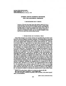
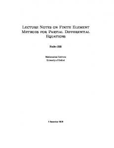
Figure 1.1: Flow-chart of the topics discussed in the present thesis.

Figure 1.2: Logical connection between the Chapters of the present thesis. The scheme of the topics discussed in the present thesis is presented in Figure 1.1 while details about the logical connection between chapters are shown in Figure 1.2. In what follows, cracks with margins free of stress are considered.

Chapter 2

FE procedures to treat crack problems Finite Element (FE) procedures, usually adopted to describe the mechanical behavior of Cauchy continua with a macroscopic crack, are critically reviewed in the present Chapter together with basic laws of crack propagation and equilibrium. Among different finite element methods, attention is focused upon the standard formulation in terms of displacement. In Section 2.1 the basic balance laws are briefly collected. Section 2.2 deals with the FE formulation of the equilibrium of cracked bodies. A sample FE analysis is presented in Section 2.3 and conclusions are in Section 2.4.

2.1

Mechanical model

A Cauchy continuum endowed with a macrocrack is considered. Following Noll [71], balance laws are deduced from the requirement that the power developed by the external interactions is indifferent under translational (Galilean) and rotational changes of spatial observers. Balances of standard forces and couples hold in the bulk, at the margins of the crack and at the tip. When one tries and describes the evolution of the crack, “fictious” interactions (called configurational ) need to be considered and balanced in the reference configuration: they are a useful tool to derive the appropriate evolution law of crack propagation in terms of the classical J -integral (see e.g. [40]).

2.1.1

Deformation and motion

Let E 3 be the three dimensional Euclidean space, elements of E 3 are points and elements of the associated vector space V are vectors (see [38]). Tensors are linear

4

2. FE procedures to treat crack problems

5

transformation between two linear spaces. A body (seen as a primitive concept) is a set of material (substantial ) elements described in the Cauchy model only through their placements in E 3 . The placement of the whole body in its reference configuration is a regular (in the sense discussed in [91] and [72]) region B0 of E 3 . A generic point of B0 is indicated with X. A standard deformation of the body is a one-to-one mapping χ : B0 → E 3 which associates to each material element placed at X in B0 its current place x =χ (X). It is assumed that χ is continuous and piecewise continuously differentiable. The map χ is also orientation preserving in the sense that its gradient ∇χ, indicated commonly with F, has positive determinant, i.e. det F > 0. The displacement u of a material point is the difference between the actual and the reference placement, namely u (X) = χ (X) − X.

(2.1)

A strain measure is introduced through the deformation tensor E, defined as E = 21 (C − I), where I is the identity tensor and C = FT F represents the CauchyGreen’s deformation tensor. Taking into account that F =∇u + I, E can be expressed ¡ ¢ as a function of the displacement field as E = 21 ∇u+∇uT + ∇uT ∇u . When the body is subject to a small deformation regime, i.e. when |∇u| :

¢ 1¡ + φ + φ− . (2.46) 2 Moreover, given two field φ1 and φ2 with the same properties of φ, [φ1 φ2 ] = [φ1 ] < [φ] = φ+ − φ−

,

=

φ2 > + < φ1 > [φ2 ]. The same relations hold even for fields taking values on some manifod (thus not necessarily scalar valued fields, but vector or tensor fields etc.), when some meaning to the difference and the product may be assigned. In some arguments illustrated below, a migrating part b (t) of B0 , varying in time, is considered. It is used to follow the evolution of the crack. The boundary of b (t) is a closed smooth curve ∂b (t) which admits an outward unit normal n and a parametric ˆ (p, t) (where p is the parameter). The velocity of a point of representation X = X ∂b (t) is

ˆ (p, t) ∂X ∂t and its normal component is indicated with U∂b n. v∂b =

(2.47)

The velocity field as seen by an observer fixed on ∂b (t) is indicated with x◦ and defined by3 x◦ = x˙ + Fv∂b Moreover, the term tip integral and the symbol [40])

Z

R tip

will be used to indicate (see

Z φ (X, t) n = lim

tip

(2.48)

r→0 ∂Dr (t)

φ (X, t) n

(2.49)

where Dr (t) is a disk of radius r centered at the crack tip and moving with it. The boundary of the disc is ∂Dr (t) and its outward unit normal is n. ˆ (p, t) , t),then by time differentiation, (2.48) follows Basically, for each X ∈ ∂b one has x =χ(X from chain rule. 3


16

Figure 2.4: Picture of the geometry used to deduce balance equations across the crack and at the tip. The Gauss theorem can be applied over the region btip (t) \Dr (t) (see Figure 2.4), then shrinking r → 0, the following generalized gradient theorem holds (see [41]) Z Z Z Z ∇φ = φn− [φ] m− φn. (2.50) b(t)

∂b(t)

b(t)∩Γ

tip

The Gauss theorem applied to a part b (t), which intersects the crack away from the tip, can be obtained from equation (2.50) neglecting simply the last integral. An analogous limit procedure allows the definition of the following generalized transport theorem (see [41]) Z Z Z Z d φ= φ˙ + φU∂b − φVtip . dt b(t) b(t) ∂b(t)∩Γ tip

(2.51)

Balance of standard forces across the crack Consider the integral balance of forces and torques (2.35) and (2.36) over a control volume bΓ intersecting the crack away from the tip. Then, by shrinking bΓ (t) to


17

bΓ (t) ∩ Γ and taking into account that, due to the continuity of the integrand, Z b0 → 0 as bΓ (t) → bΓ (t) ∩ Γ, (2.52) bΓ (t)

the following balance holds:

Z [S] m = 0.

(2.53)

[S] m = 0 on Γ,

(2.54)

bΓ (t)∩Γ

The arbitrariness of bΓ implies that

which states the continuity across the crack of the normal component of the tension obtained multiplying the first Piola-Kirchhoff stress tensor by the normal. Balance of standard forces at the crack tip Balance equations at the crack tip are obtained by considering a disk Dr (t) centered at Z and writing the integral balance (2.35) as Z Z b0 + Sn + btip 0 = 0, Dr (t)

(2.55)

∂Dr (t)

where an additional inertial term acting upon the tip of the crack has been added to account for possible inertial contributions at the tip (i.e. btip 0 is assumed to be of only inertial nature). Then, shrinking Dr (t) to the tip, by letting r → 0, and taking into account the continuity of b0 , the following balance follows4 : Z tip b0 + Sn = 0

(2.56)

tip

Now it is necessary to identify explicitly the inertial term btip 0 , just formally introduced, in terms of the rates connected with the kinematics of the crack. Preliminary, note that, from equation (2.41), the following balance of inertial forces on an arbitrary part b far from the crack follows: Z b

bin 0

d =− dt

Z ρx˙

(2.57)

b

To identify the inertial term btip 0 consider a part btip (t) around the crack tip. If one decides to apply (2.57) to a part btip (t) around the tip, migrating to follow the 4

Since b0 is continuous over Dr (t), lim

R

r→0 Dr (t)

b0 = 0.


18

crack evolution, one needs to add btip on the right-hand side term of (2.57) and the flow of momentum through the moving boundary5 , i.e. Z Z Z d tip in b0 + b0 = − ρx+ ˙ ρxU ˙ ∂b dt btip (t) ∂btip (t) btip (t)

(2.58)

then, shrinking diam (btip (t)) → 0 and taking into account equation (2.42), the following expression holds: Z btip 0 =

tip

Z ρx˙ (vtip · n) =

Finally, equation (2.56) reduces to Z Z Sn+ tip

tip

tip

ρxV ˙ tip .

ρxV ˙ tip = 0.

(2.59)

(2.60)

Physical evidence justifies the assumption that the stress be bounded up to the R tip. This implies that tip Sn = 0 (as a consequence of the theorem of the mean value) and equation (2.60) reduces to

Z tip

ρxV ˙ tip = 0

(2.61)

In other words, the velocity of the crack, when the stress at the crack tip is bounded, has always a finite value. Typically, equation (2.61) is considered as an assumption, R and tip Sn = 0 follows (see [32]). Interactions due to the crack growth: configurational forces The crack growth is a phenomenon that occurs in the actual configuration of the body together with its deformation. In the reference configuration the crack has a growing image Γ (t). Thus, the growth of Γ constitutes an independent kinematics in B0 to which explicit interactions (defined in B0 ) must be associated (to each kinematic mechanism, in fact, interactions are commonly associated to measure the power necessary to develop that mechanism). Since the kinematics of Γ in the reference configuration is only apparent because Γ is not a material surface (it is only the image of the crack under the inverse motion), the interactions associated to that kinematics (called also configurational ) are apparent and must be expressed in terms of the standard interactions that are generated in the actual configuration B and can be pulled back in B0 through the Piola transformation (e.g. the Piola-Kirchhoff stress S is the pull-back i.e. the image in B0 - of the Cauchy stress T living in B). Configurational forces in B0 are expressed through (see [40]): R Basically, one should consider the flow ∂b (t) ρxU ˙ ∂b , where U∂b is the amplitude of the normal tip component of the velocity of the boundary, because btip is taken to vary in time, on the contrary of b of (2.57) which is fixed. 5


19

• bulk measures of interaction described through a stress tensor P, an internal force vector g and an external force vector e; • line measures of interaction described through a line stress σt (with σ a constant because any piece of Γ far from the tip does not increase its length during the crack growth) and an internal force along Γ, namely gΓ ; • point measures of interaction described through a vector of internal tip forces gtip and a vector etip collecting inertial contributions at the tip. The balance of configurational forces can be obtained following a procedure used in [40] and[39], i.e. by imposing the invariance of the power with respect to a change from a fixed material observer to a moving material observer. For the sake of simplicity, such procedure is here skipped and balance of configurational forces are only reported (for more details see [41] and [40]). The pointwise balance of configurational forces in the bulk B0 , across the crack Γ and at the crack tip are DivP+g + e = 0 in B0 ,

(2.62)

[P] m + gΓ = 0 along Γ, Z gtip + etip − σtZ + Pn = 0 at the tip.

(2.63) (2.64)

tip

The term etip can be characterized explicitly by considering a part btip (t) which contains the tip and imposing that the rate of the kinetic energy in btip (t) must be equal to the power of the inertial forces, for any choice of the rates involved, namely Z Z Z d 1 1 ρx˙ · x− ˙ ρx˙ · xU ˙ ∂b(t) + bin ˙ + btip ˜tip + etip · vtip = 0 0 ·x 0 ·v dt btip (t) 2 2 ∂btip (t) btip (t) (2.65) Then, by shrinking btip (t) up to the tip, taking into account equation (2.59) and R R considering that btip (t) (·) U∂b(t) → tip (·) (vtip · n) as btip (t) → Z, the following relation holds for any choice of vtip Z Z 1 −vtip · ρ (x˙ · x) ˙ n + vtip · (ρx˙ · v ˜tip ) n + etip · vtip = 0 tip 2 tip

(2.66)

The arbitrariness of vtip implies Z etip = where krel = 1 vtip 2 ρ˜

·v ˜tip =

1 ˙ −v ˜tip |. 2 ρ |x 1 ˙ · x−ρ ˙ x˙ · 2 ρx

tip

krel n

(2.67)

To obtain equation (2.67), one uses the identity krel − v ˜tip .


20

Consequences of the mechanical dissipation inequality in the bulk To identify explicitly the configurational interactions in terms of the standard stress and bulk forces, one needs to use (see [40], [39]) an isothermal version of the ClausiusDuhem inequality (thus a mechanical dissipation inequality) which states that, for any part b (t) and any choice of the rates involved, d {free energy} − {power developed on b} ≤ 0 dt

(2.68)

Let b (t) be an evolving part in B0 far from the crack, equation (2.68) reduces to Z Z Z d ψ− b0 ·x− ˙ Sn · x◦ + Pn · v∂b(t) ≤ 0 (2.69) dt b(t) b(t) ∂b(t) where the term Sn · x◦ represents the power developed by deformational forces on ∂b (t), taking into account both its material ((in B0 the boundary ∂b (t) evolves) and actual kinematic and the term Pn · v∂b(t) represents the power developed by the configurational stress on ∂b (t) taking into account its material kinematic, because P lives only in B0 . Z

By a standard transport theorem, equation (2.69) becomes Z Z Z ¢ ¡ ¡ T ¢ ψ˙ − ψ (v∂b · n) − b0 ·x− ˙ Sn · x+ ˙ F T + P n · v∂b ≤ 0 (2.70)

b(t)

∂b(t)

b(t)

∂b(t)

In [39], it is noted that the parametrization of ∂b (t) can be chosen arbitrarily without any physical stringent motivation; then it is suggested that a natural requirement is to impose that (2.70) be independent of the parametrization of ∂b (t). The term depending on such parametrization is only the component of v∂b tangential to ∂b (t). ¡ ¢ Then it follows that one must impose that the vector FT T + P n must be purely ¡ ¢ normal to ∂b (t), i.e. FT T + P n =πn (with π an undetermined scalar at this stage). This implies P = πI − FT T.

(2.71)

Equation (2.71) can be substituted again in equation (2.70) obtaining Z Z Z Z ψ˙ − (ψ − π) U∂b − b0 ·x− ˙ Sn · x˙ ≤ 0 b(t)

∂b(t)

b(t)

(2.72)

∂b(t)

which must be valid for any choice of the rates involved. This implies that the configurational term π coincides with the free energy: π = ψ.

(2.73)

The last expression allow us to identify explicitly the configurational stress P through P =ψI − FT S

(2.74)


21

which is the expression of the celebrated Eshelby’s tensor. By substituting (2.74) into (2.62) and taking into account (2.37), one obtains the following explicit expression of g and e (see [39], [40]): ¡ ¢ g = −∇ψ + ∇FT S

(2.75)

e = −FT b

(2.76)

ˆ (X, F), applying the Gauss theorem and taking into By assuming that ψ = ψ account equations (2.73) and (2.37), equation (2.72) reduces to Z ˙ ≤ 0, (∂F ψ − S) ·F

(2.77)

b(t)

which must be valid for any choice of the rate and any part b (t). This implies that S =∂F ψ.

(2.78)

Since ∇ψ = ∂X ψ + ∂F ψ∇F, thanks to (2.78), equation (2.75) reduces to g = −∂X ψ

(2.79)

which vanishes identically in homogeneous materials. Consequences of the mechanical dissipation inequality across the crack Consider a part bΓ (t) that intersect the crack away from the tip. Equation (2.68) reduces to ÃZ ! Z Z Z Z d ◦ ψ+ η − b · x− ˙ Sn · x +Pn · v∂b − σt · v∂b ≤ 0 dt bΓ (t) bΓ (t)∩Γ bΓ (t) bΓ (t) ∂bΓ (t)∩Γ (2.80) where η represent a constant free energy line density. With the use of (2.48) and (2.74), equation (2.80) can be written as ÃZ ! Z Z Z Z d ψ+ η − b · x− ˙ Sn · x+π ˙ (n · v∂b )− σt·v∂b ≤ 0 dt bΓ (t) bΓ (t)∩Γ bΓ (t) bΓ (t) ∂bΓ (t)∩Γ (2.81) Then, shrinking bΓ (t) to Γ, the following relation holds: Z Z (η − σ) t · v∂b − [Sm · x] ˙ ≤0 bΓ (t)∩Γ

(2.82)

bΓ (t)∩Γ

which must be valid for any choice of the velocity fields. This implies that η = σ.

(2.83)


22

Moreover, thanks to (2.83) and the arbitrariness of b, equation (2.82) reduces to [Sm · x] ˙ ≥ 0. Since [Sm · x] ˙ =< S > m· [x] ˙ + [S] m· < x˙ > and [S] m = 0, it follows that < S > m· [x] ˙ ≥0

(2.84)

which is always zero when the crack faces are unstressed (i.e. when < S > m = 0). Consequences of the mechanical dissipation inequality at the crack tip Consider a disk Dr (t) centered at the crack tip and evolving following it. Equation (2.68) assumes the following form on Dr (t): ÃZ ! Z Z d ψ+ η − b0 ·x+ ˙ dt Dr (t) Dr (t)∩Γ Dr (t) Z − ∂Dr (t)

(Sn · x◦ +Pn · v∂D ) − σ A (tA · vA ) − etip · vtip ≤ 0

(2.85)

³R ´ R R d ψ + η → 0 and the term Dr (t) b0 ·x˙ → 0 (see [40]). As r → 0, dt D (t) D (t)∩Γ r r R Moreover, ∂Dr (t) Sn · x◦ → 0 because the boundary of the disk has the velocity of the

I tip (i.e. x◦ ≡ xI ˜tip (see [40]) and tip ) and, as r → 0, xtip → v

Z lim

Z

r→0 ∂D(t)

Sn · x◦ = v ˜tip ·

Sn = 0

(2.86)

tip

for the boundedness of the stress at the tip. As a consequence, equation (2.85) reduces to

Z −vtip ·

tip

Pn − σ tip tZ · vtip − etip · vtip ≤ 0

(2.87)

By substituting equation (2.64) in (2.87), one reduces the mechanical dissipation inequality at the crack tip to gtip · vtip ≤ 0

(2.88)

which shows that gtip is a dissipative force, usually associated with “the breaking of bonds at the crack tip, that opposes motion of the tip” (see [41] pag. ; see also [32]). Equation (2.88) admits the solution gtip = −atip vtip = −atip Vtip tZ

(2.89)

where atip is a positive defined function of the state variable, which can be assigned constitutively (see [41],[32]).


23

The crack driving force and the J integral By taking into account (2.67) and (2.89), equation (2.64) can be written in the form ¶ ¶ Z µµ 1 −atip Vtip tZ − σ tip tZ + (2.90) ψ+ ρx˙ · x˙ I − FT S n = 0, 2 tip or, alternatively, as gtip − σ tip tZ + j = 0, where j =

¢ ¢ ¡¡ T 1 ρ x ˙ · x ˙ I − F S n repreψ+ 2 tip

R

sents a traction at the crack tip whose component along the direction of propagation of the crack tZ is indicated with Jdyn = j·tZ and called dynamic J-integral. Commonly, the product gtip · tZ is indicated with −G and called dynamic energy release rate. Then, by multiplying (2.90) by tZ , it follows that G = Jdyn − σ tip .

(2.91)

The local dissipation inequality (2.88) then reduces to GVtip ≤ 0.

(2.92)

Once some constitutive prescriptions is assigned to atip , equations (2.91) and (2.89) furnish the velocity of propagation of the crack, namely Vtip =

1 (Jdyn − σ tip ) . atip

(2.93)

When the inertial forces are negligible, the study of the crack propagation is restricted to the quasi-static case, and Jdyn reduces to Z Z ¡ ¢ Jq−st = tZ · Pn =tZ · ψI − FT S n. tip

Equation (2.93) becomes Vtip =

(2.94)

tip

1 atip

(Jq−st − σ tip ) and furnishes the velocity of

propagation of the crack in absence of inertial effects. It is well known that the Jq−st is path independent when (i) the material is homogeneous (g = 0), (ii) the faces of the cracks are traction free (< S > m = 0) and (iii) the crack itself is straight (see Rice; see also [40] and [32]. The proof can be developed by noting that, if Jq−st is path independent, then for any arbitrary disc Dr centered at the tip and of radius r, the following identity should hold: Z Z tZ · Pn =tZ · Pn. ∂Dr

From equation (2.50), it follows that Z Z Z tZ · Pn =tZ · DivP+tZ · ∂Dr

Dr

(2.95)

tip

Dr ∩Γ

Z [P] m+tZ ·

Pn. tip

(2.96)


24

Moreover, taking into account equation (2.62) in the quasi-static regime (e = 0) and the assumption that the material is homogeneous (g = 0), the formula (2.96) changes as Z Z tZ · Pn =tZ · ∂Dr

Dr ∩Γ

¡ £ ¤ ¢ [ψ] m− FT < S > m− < FT > [S] m +tZ ·

Z Pn. (2.97) tip

However, the assumption that the faces of the crack are traction free implies < S > m = 0 while the balance across the crack prescribes that [S] m = 0 (see 2.54). R Moreover, tZ · Dr ∩Γ [ψ] m = 0 for straight crack, because tZ is orthogonal to m. As a consequence, (2.95) follows.

2.2

Numerical approximation: Finite Element Method

Consider a body that occupies the region B0 in its crack free reference configuration and is endowed with a crack in its current configuration which does not intersect the boundary. The image of the crack in B0 by inverse motion is the curve Γ (Figure 2.5). With reference to Figure 2.5, the boundary ∂B0 of B0 is divided in two portions ∂B0u and ∂B0t such that ∂B0 = ∂B0u ∪ ∂B0t

(2.98)

∂B0u ∩ ∂B0t = ∅

(2.99)

The equilibrium boundary value problem has the following strong formulation (balance equations are briefly recalled): (s) given b0 : B0 → R3 , ¯ t :∂B0t → R3 and u ¯ :∂B0u → R3 , find u such that DivS + b0 = 0 on B0 [S] m =0 across Γ u= u ¯ on ∂B0u

(balance in the bulk)

(stress continuity condition)

(displacement boundary condition)

Sn=¯ t on ∂B0t

(traction boundary conditions)

(2.100a) (2.100b) (2.100c) (2.100d)

In addition to the above relations, the balance of torques states that SFT = FST .

2.2.1

From a strong form to a weak form

Let C be a space of vector valued fields defined on B0 , suffciently smooth far from Γ. The space of trial functions U is defined by U={u ∈ C | u = u ¯ on ∂B0u }

(2.101)


25

Figure 2.5: Displacement and traction boundary conditions. and represents the space of the kinematically admissible displacement fields. The trial functions satisfy the continuity condition required for compatibility and the displacement boundary conditions. The space of test functions U0 is defined as U0 ={δv ∈ C| δv =0 on ∂B0u }

(2.102)

The test functions δv are sometimes called virtual displacements and vanish where the trial functions satisfy the displacement boundary conditions. The first step in constructing a weak form of the boundary value problem consists in multiplying the equilibrium equation (2.37) with a test function and integrating them over the whole domain. One then obtains Z δv· (DivS + b0 ) = 0 B0

∀δv ∈U0 .

(2.103)


26

The application of the Gauss theorem gives Z Z Z Z δv · Sn− ∇ (δv) ·S− δv· [S] m+ ∂B0

B0

Γ

B0

δv · b0 = 0

∀δv ∈U0

(2.104)

then, by substituting the boundary conditions and the stress continuity condition, it follows that Z B0

Z (∇ (δv) ·S−δv·b0 ) −

δv · ¯ t=0 ∂B0t

∀δv ∈U0 .

(2.105)

The weak form (w) of the boundary value problem (s) then arise: given b0 : B0 → R3 , ¯ t :∂B0 → R3 and u ¯ :∂B0 → R3 , find u∈ U such that for all δv ∈U0 (w)

n R

B0 (∇ (δv) ·S−δv·b0 ) −

R

¯ ∂B0t δv · t = 0

o .

(2.106)

The strong and the weak formulation illustrated above are equivalent (see for the proof [46] for linear elasto-statics and [7] for non-linear dynamics, but one can simply think to the principle of virtual work). If the body undergoes a small deformation regime (|∇u| 0

(3.10)

Note that the Heaviside function has been modified to be symmetric across the crack.

3. X-FEM: a numerical method to treat discontinuous solutions. The formulation of an higher order extended finite element.

41

Figure 3.6: Enriched nodes in a structured (right picture) and an unstructured (left picture) mesh. It is worth noting that, as a consequence of equation (3.9), the I -th nodal value of the approximate displacement field is uh (XI ) = uI

(3.11)

which coincides with the nodal value of the standard displacement field. Equation 3.11 can be obtained taking into account the standard property of the shape function, which states that NJ (XI ) = δ IJ

(3.12)

where δ IJ is the Kcroneker delta. The property expressed by equation (3.11) must be considered when essential boundary conditions are imposed over enriched nodes. ˜I (X) are In equation (3.9), the shape functions NI (X) are quadratic whereas N linear. The choice of different shape functions between the uhcon and uhdis is due to a property of the partition of unity used in constructing the finite elements in the region where enriched elements blend to non-enriched elements. A detailed discussion about this argument can be found in [21]. For reader’s convenience, the parent coordinates for a three and six nodes triangle are shown in Figure 3.7, while in Table 3.1 their explicit expressions are reported. In equation (3.9), the vector columns uI are the standard nodal displacements and aJ and bαK are additional nodal degrees of freedom. In the same equation, the functions F α (r, θ) forms the basis for the Westergaard field for the crack tip, which are defined in [31] as

√ θ r sin 2 √ θ F 2 (r, θ) = r cos 2 F 1 (r, θ) =

(3.13) (3.14)


N1 N2 N3 N4 N5 N6

Linear 1−ξ−η ξ η -

42

Quadratic 1 − 3ξ − 3η + 4ξη + 2ξ 2 + 2η 2 ξ (2ξ − 1) η (2η − 1) 4ξ (1 − η − ξ) 4ηξ 4η (1 − η − ξ)

Table 3.1: Linear and quadratic shape functions in terms of parent coordinate (ξ, η) for triangles.

Figure 3.7: Parent coordinates (ξ, η) for a six nodes triangle. √ θ r sin sin θ (3.15) 2 √ θ (3.16) F 4 (r, θ) = r cos sin θ 2 where r = |X − Z| = g(X), with reference, e.g., to a situation similar to figure 3.6 but F 3 (r, θ) =

with a straight crack, for which Z is the place of the tip. The functions F α (r, θ) are called branch functions, their plot is shown in Figure 3.8, in 2D view, and in Figure 3.9, in the 3D view. It is worth noting that the function in (3.13) is discontinuous across the crack face, while the other three functions (3.14)-(3.16) are continuous, as it is shown in Figures 3.8 and 3.9. This means that F 1 represents the discontinuity near the tip, while the other three functions span the Westergaard solution near the crack tip and improve the numerical accuracy.


43

Figure 3.8: 2D view of the branch functions used to enrich nodes that belong to N T ip . To take into account a possible curvature of the crack, two definitions of θ are used. Let tI be a vector tangent to the crack at a given point. We define θ as follows: at a point x, if t · ∇g ≤ 0 we use the regular polar angle. If t · ∇g > 0, θ is computed by: −f arctan(θ) = p . g2 − f 2

(3.17)

The minus sign in (3.17) is needed to reconcile this definition with the regular polar coordinates (see discussion in [10]). One must be careful with the sign of f , which has to be reversed to be consistent with the local polar orientation at the second tip of a crack, when one considers a crack not intersecting the boundary of the body in any point. Another definition for θ could be given by arcsin(θ) =

f . g

(3.18)

To clarify the character of the approximation of the Heaviside term in (3.9), the enriched shape functions for a 3-node quadratic element in one dimension are shown


44

Figure 3.9: 3D view of the branch functions used to enrich nodes that belong to N T ip . ˜I vanishes in Figure 3.11. The product of the enrichment function at node I with N always at all nodes. When the discontinuity is near the end nodes, as shown in Figure 3.11d, the approximation must be modified because the two basis functions are almost identical, as it can be seen by comparing Figure 3.11d with Figure 3.11a. The stiffness matrix will then tend to be ill-conditioned. In these situations it is necessary to shift the enrichment to the subsequent element. For midpoint nodes the enrichment differs from the nodal shape function even when the discontinuity is near the midpoint node, so no modifications are needed (see Figures 3.11e and 3.11g,). By substituting the displacement approximation (3.9) into the strain definition


45

Figure 3.10: Orientation at the crack tip to define the interior of the crack and the domain beyond the crack. (2.2) the following expression for the strain follows: 

¯u = ε = B¯ h

h

BuI

BaJ

Bb1 K

Bb2 K

BbK

Bb4 K

   i      

uI



 aJ   b1K    , with 2 bK   b3K   4 bK

I = 1...N J = 1...N cr K = 1...N T IP

(3.19) ¯ ¯ where B is a strain-displacement matrix. The matrix B has the following explicit forms:

  BuI = 

NI,x 0 NI,y

  BaJ = 

¯ ¯ Bbα K¯

α=1,2,3,4

˜J (H − H(f (XJ )))),x (N 0

0



 NI,y  NI,x

(3.20)

0



˜J (H − H(f (XJ )))),y  (N  ˜J (H − H(f (XJ )))),x (N

˜J (H − H(f (XJ )))),y (N   ˜K (F α − F α (XK ))),x (N 0 K K  ˜K (F α − F α (XK ))),y  = 0 (N , K K ˜K (F α − F α (XK ))),y (N ˜K (K α − F α (XK ))),x (N K K K K

(3.21)

(3.22)

where the coma indicates derivation with respect to the indicated variable. By substituting the displacement (3.9) and the strain approximation (3.19) into the weak form of the equilibrium problem (2.106), the following discrete system of equations is obtained: Kp = f ext

(3.23)


46

Figure 3.11: Enriched shape functions for a three nodes one dimensional element: the first shape function is modified as shown in case (c) when the discontinuity is close to node 2 and as in case (d) when it is close to node 1; the second shape function is instead modified as shown in case (g) when the discontinuity is close to node 2. where f ext is the vector of external loads, p is the vector of nodal unknowns and K the stiffness matrix given by

Z ¯ T CB ¯ B

K=

(3.24)

Bh

The expression of the vector f ext of the external forces is b1 b2 b3 b4 f ext = {fIu ; fJa ; fK ; fK ; fK ; fK }

where

Z fIu

= ∂Bt

Z NI ¯ t+

B

NI b

represents the standard nodal external forces and Z Z a ˜ ˜J (H − H(f (XJ )))b ¯ fJ = NJ (H − H(f (XJ )))t + N ∂Bt

(3.25)

B

(3.26)

(3.27)

3. X-FEM: a numerical method to treat discontinuous solutions. The formulation of an higher order extended finite element. Z

¯

bα ¯ fK ¯

α=1,2,3,4

= ∂Bt

47

Z ˜K (F α − F α (XK ))¯ N t+

B

˜K (F α − F α (XK ))b N

(3.28)

(with α = 1, 2, 3, 4) are additional nodal forces associated with the enriched nodes. As in the case of standard finite element methods, the essential boundary conditions are enforced directly on p which includes the additional enriched degrees of freedom.

3.3.3

Element integration

The integration of the stiffness matrix (3.24) and nodal forces (3.26 - 3.28) in the elements which are not enriched follows the same procedure used in the standard FEM analysis. A special procedure, based upon the creation of subelements by triangular partitioning, is instead required when the integration is performed over enriched elements. Elements completely cut by the crack are distinguished by those that are slit by the crack tip. The triangular partitioning for the element of the former group is shown in Figure 3.12. For each triangle three further triangles are created. In each of these new elements, 13 points for Gaussian quadrature are used.

Crack

line−path of the crack

line joining to one sommet

Figure 3.12: Delaunay partitioning of an element cut by a crack. The elements containing the crack tips are instead partitioned as described in Figure 3.13. Each triangle is subdivided in four triangles and in each new triangle 13 Gauss points for quadrature integration are used. The increase in computational cost is not significant.

3. X-FEM: a numerical method to treat discontinuous solutions. The formulation of an higher order extended finite element. Crack tip Crack

48

Crack tip position

Figure 3.13: Delaunay partitioning of an element containing the crack tip.

3.4

Numerical examples

This Section deals with the testing of the six node triangular element developed in the setting of X-FEM and presented above. Such kind of element is referred to as quadratic X-FEM. Several fracture mechanics problems are considered and numerical solutions are compared with closed form solutions available in literature. It is worth recalling that the six node X-FEM element uses quadratic interpolants for the displacement approximation and linear interpolants for the partition of unity and the blending. Crack opening displacements, the energy error and stress intensity factors are calculated and compared with closed form and benchmark solutions. These results are also compared to an X-FEM formulation which uses only linear interpolants, referred to as the linear X-FEM formulation. Moreover, the problem of the infinite plate, already tackled in Chapter 1 by using standard FEM, is again analyzed using X-FEM, in order to propose a comparison between numerical results obtained with standard FEM and X-FEM. It is worth noting that in the convergence studies reported below the Westergard enrichment was applied only in the element containing the crack tip whose size decreased as the mesh was refined. Morever, it should be pointed out that, in the present chapter, the numerical simulations developed with the X-FEM take into account problems with single crack. In this case the number of enriched nodes is small with respect to the total number of mesh nodes and the computational cost does not increase significantly with respect to a standard FEM procedure.

3.4.1

Infinite plate under remote load

Consider once again the problem of the infinite plate containing a straight crack of length 2a and loaded by a remote tensile stress t already illustrated in Chapter 1.


49

A closed form solution for this problem in terms of stress is expressed by equations (2.117)-(2.119), while equations (2.120)-(2.121) represent the solution in terms of displacements. Recall that the closed form solution referred to is assumed to be valid in a small region around the crack tip indicated with ABCD in Figure 2.6.

B

C

A

D

Figure 3.14: Discretization around the crack tip of an infinite plate loaded by a remote stress. Nodes labelled with a circle are enriched with a step function and nodes indicated with a square are enriched with the Westergaard functions.

Comparison between linear and quadratic X-FEM In the X-FE procedure, the region ABCD of Figure 2.6 is discretized as shown in Figure 3.14. Num Node 100 196 400 576 1600

ln(Energy Error) -1.1644 -1.3436 -1.6057 -1.6926 -1.7897

Energy Error 0.3121 0.2609 0.2007 0.1840 0.1670

Error of J integral 0.0718 0.0629 0.0153 0.0111 0.0080

Table 3.2: Infinite plate of Figure 2.6 solved with a linear X-FEM. All simulations are performed with a = 100 mm and t = 104 N/mm2 on a square mesh with sides of length 10 mm (see Figure 3.14).

3. X-FEM: a numerical method to treat discontinuous solutions. The formulation of an higher order extended finite element. Num Node 221 421 1201 2381 3613

ln(Energy Error) -2.2377 -2.3651 -2.4686 -2.4866 -2.8467

Energy Error 0.1067 0.0939 0.0847 0.0832 0.0580

50

Error of J integral 0.0114 0.0044 0.0030 0.0015 0.0015

Table 3.3: Infinite plate of Figure 2.6 solved with an hybrid X-FEM. −1

0

10

10

Linear Element: Convergence rate= −0.90311 Quadratic Element: Convergence rate= −0.66871

ln(Error on J integral)

ln(Energy Error)

Linear Element: Convergence rate= −0.23656 Quadratic Element: Convergence rate= −0.1727

−1

10

−3

−2

10

−2

10

10 2

10

3

10

4

10

ln(N)

2

10

3

10

ln(N)

Figure 3.15: Energy norm (right) and J integral error (left) convergence for linear and quadratic elements in X-FEM. N is the number of nodes. Numerical simulations were performed prescribing on the entire boundary of the mesh the displacements by using equations (2.120)-(2.121). The normalized energy error norm is then calculated by equation (2.124) and compared with that obtained from the exact solution. In tables 3.2 and 3.3 the energy error and the error on the J integral, for linear and hybrid X-FEM elements respectively, are reported. Moreover, in Figure 3.15(left), the convergence rates of the error in terms of energy for the linear and the quadratic X-FEM are compared. The calculations of the J integral are performed following the procedure recalled in Appendix A. In Figure 3.15 (right) the convergence of the calcualtion of the J-integral is shown for the linear and hybrid X-FEM. The crack opening displacement (COD) along the crack can be calculated directly from the enriched finite element approximation (3.9) by using the following expression h i ¡ ¢ ¡ ¢ uh = uh X+ − uh X− (3.29) £ ¤ In developing the explicit expression for uh it must be taken into account that only two discontinuous terms of expression (3.9) remain: they are the jump across the

4

10


51

Crack Openeing Displacement − Linear element

0.2

Exact Numerical 0.1

0

0

0.5

1

6

1.5 2 2.5 3 3.5 Crack Openeing Displacement − Hybrid element

4

4.5

5

Exact Numerical

4 2 0

0

0.5

1 1.5 2 2.5 3 3.5 4 X component of displacement along Crack Section − Linear element

0.02

4.5

5

Exact Numerical

0.01 0 −0.01

0

1

2 3 4 5 6 7 8 X component of displacement Crack Section − Hybrid element

1

9

10

Exact Numerical

0.5 0 −0.5

0

1

2

3

4

5 X

6

7

8

9

10

Figure 3.16: Simulations with a coarse mesh: in the first two figures above, the Crack Opening Displacement, calculated with a linear element (top figure) and an hybrid element (bottom figure), is compared with that one obtained from the exact solution; in the two figures below, an analogous comparison is developed by using the tangential component of displacement along the crack. crack faces X

³ ³ ¡ ³ ¡ X ¢´ ¢´´ ˜I ˜I H f h X+ − H f h X− N aI = 2 aI N

I∈N Cr

(3.30)

I∈N Cr

and that one at the crack tip X

¡ ¡ ¢ ¡ ¢¢ √ X ˜I F 1 r, θ+ − F 1 r, θ− bI = 2 r ˜I N bI N

I∈N Cr

(3.31)

I∈N tip

when θ+ = π and θ− = −π are considered. It is worth noting that only the first branch function contributes to the jump at the crack tip (3.31).


52

Crack Openeing Displacement − Linear element 0.2 Exact Numerical 0.1

0

0

0.5

1

1.5 Openeing 2 Displacement 2.5 3 3.5 Crack − Hybrid element

4

4.5

5

6 Exact Numerical

4 2 0

0

0.5

1 1.5 2 2.5 Crack Section 3 4 X component of displacement along −3.5 Linear element

4.5

5

0.02 0.01 Exact Numerical

0 −0.01

0

1

2 3of displacement 4 5 Crack Section 6 8 X component along −7 Hybrid element

9

10

1 0.5 Exact Numerical

0 −0.5

0

1

2

3

4

5 X

6

7

8

9

10

Figure 3.17: Simulations with a refined mesh (compare with Figure 3.16): in the first two figures above, the Crack Opening Displacement, calculated with a linear element (top figure) and an hybrid element (bottom figure), is compared with that one obtained from the exact solution; in the two figures below, an analogous comparison is developed by using the tangential component of displacement along the crack. Then, by considering (3.30) and (3.31), the following approximate expression of the COD holds

h i X √ X ˜I + 2 r ˜I uh = 2 aI N bI N I∈N Cr

(3.32)

I∈N tip

Analogously, the closed form expression for the COD in an homogeneous and isotropic body is [u] = u+ − u− , where [u] is the jump across the crack. It can ¡ ¢ be deduced from equation (2.121) by considering that u+ = uy r, θ+ = π and u− = ¡ ¢ uy r, θ− = −π . It follows that r [u] = 8

r KI (1 − ν 2 ) 2π E

(3.33)


53

Figure 3.16 compares the COD and the horizontal component of displacement for the linear and the quadratic elements respectively with the exact values deduced from the closed form solution. The numerical results for linear and hybrid X-FEM are relative to the same structured mesh of 100 triangular elements. It is important to note that the horizontal component of the displacement, which is less accurate than the vertical one in both the simulations, has maximum value almost ten times less than the maximum value of the crack opening displacement. The simulations performed with the hybrid element (see Section 3.3) are more accurate than that done with the linear element. In Figure 3.17, an analogous analysis is performed with a refined mesh: both the linear and the hybrid elements increment the accuracy and the hybrid element gives, once again, better numerical approximation.


54

Comparison between quadratic FEM and quadratic X-FEM 0

10

ln(Energy Error)

FEM Quadratic Element: Convergence rate= −0.26462 X−FEM Hybrid Element: Convergence rate= −0.26525

−1

10

−2

10

2

10

3

4

10

10

5

10

ln(N)

Figure 3.18: Energy error as a function of number of nodes N for quadratic FEM and quadratic X-FEM. The problem of the infinite plate was already illustrated in Chapter 1 and solved with a FEM analysis using a six node triangular element. The same problem has been tackled in the present Chapter with an X-FEM analysis. One may then compare the results of the FE with those of X-FEM analysis. The error in terms of the energy norm for a quadratic FEM and a quadratic XFEM is shown in Figure 3.18. X-FEM analysis produces better numerical results and almost the same rate of convergence as the number of nodes increase. Analogously, numerical results between quadratic FEM and X-FEM, by computing the error on the J-integral are compared in Figure 3.19. Moreover, in this case, X-FEM analysis shows better approximation and a higher rate of convergence. It is worth noting that either FEM or X-FEM analysis are performed by using an unstructured mesh made of six nodes triangular elements. The increment of number of nodes is obtained refining the mesh in the whole domain (see Figure 2.6), even if it


55

Unstructured mesh

−1

10

FEM Quadratic Element: Convergence rate= −0.513 X−FEM Hybrid Element: Convergence rate= −1.1472

−2

ln(Error on J integral)

10

−3

10

−4

10

2

10

3

4

10

10

5

10

ln(N)

Figure 3.19: J integral error as a function of number of nodes N for quadratic FEM and quadratic X-FEM. is a common practice in FEM analysis to refine the mesh only in the region where it is known a priori that the solution could have a singularity.


3.4.2

56

Edge crack under tension

Consider a plate loaded by a tension t = 1.0 psi over the top and bottom edges as shown in Figure 3.20.

Figure 3.20: Plate with edge crack under tension. A reference frame (x, y) is centered in the bottom left corner of the mesh with the x -axis and the y- axis placed along the horizontal and vertical edges, oriented along the edges themselves, respectively. The body is fixed at the bottom right corner, and clamped at the bottom left corner. The material parameters are 103 psi for Young’s modulus and 0.3 for Poisson’s ratio. The exact value of the stress intensity factor KI is given by (see [29], page 49)

√ (3.34) KI = t πaC, ¡a¢ where a is the crack length, C = C b an empirical function and b the plate width. The numerical value of KI can be deduced by equation (2.122) through the value of the J-integral, calculated with the procedure illustrated in Appendix A. For a/b ≤ 0.6,


57

the function C is (see [29], page 49) C

³a´ b

= 1.12 − 0.231

³a´ b

+ 10.55

³ a ´2 b

− 21.72

³ a ´3 b

+ 30.39

³ a ´4 b

(3.35)

The same type of structured mesh as shown in Figure 3.14 has been used except that the body is 1 × 2 and the mesh is 12 × 12. In Table 3.4, the numerical results obtained in this Chapter are compared with the ones of EFG (Element Free Galerkin) method presented in [9]. crack length 0.21 0.22 0.23 0.24 0.28 0.50

KI XFEM (linear) 1.0616 1.1000 1.1321 1.1558 1.3783 3.1299

KI XFEM (quadratic) 1.1243 1.1691 1.2187 1.2707 1.4760 3.5064

KI EFG Belytschko et al. [9] 1.1401 1.1779 1.2487 1.2807 1.5036 3.5512

KI exact 1.1341 1.1816 1.2303 1.2788 1.4935 3.5423

Table 3.4: Stress intensity factors computed by quadratic X-FEM compared with EFG. For EFG, the number of cells has been 10 × 10 and a 5 × 5 Gauss quadrature has been used in all cells except the two around the crack tip, where a 9 × 9 Gauss quadrature has been adopted. Quadratic X-FEM seems to behave as well as EFG Method. While EFG Method tends to overestimate the stress intensity factors, the quadratic X-FEM tends to underestimate the exact result.


3.4.3

58

Edge crack under shear stress

τ=1

L=16 a = 3.5

W=7 Figure 3.21: Discretization of the edge crack problem under shear. Consider a plate (of homogeneous and isotropic material) clamped on the bottom and loaded by a uniformly distributed shear traction τ = 1.0 psi over the top edge (see Figure 3.21 where the mesh used in the numerical calculations is also shown). The material parameters adopted for the numerical simulations are 3 · 107 psi for Young’s modulus E and 0.25 for Poisson’s ratio ν. The reference mixed mode stress intensity factors, calculated by a boundary collocation method, as given in [95] and [89] are KI

= 34.0

KII

= 4.55

√ psi in √ psi in

In mixed mode crack problems, like the present one, the stress intensity factors KI and


59

0

10

ln(Error on Keq)

Keq − Linear Element Keq − Quadratic Element

−1

10

−2

10

2

3

10

4

10

10

ln(Number of Nodes)

Figure 3.22: Convergence for edge crack under shear. Keq is computed from the J-integral. 0

0

10

10

K2 − Linear Element K2 − Quadratic Element

ln(Error on K2)

ln(Error on K1)

K1 − Linear Element K1 − Quadratic Element

−1

10

−2

10

−3

−2

10

−1

10

2

10

3

4

10

10

ln(Number of Nodes)

10

2

10

3

10

ln(Number of Nodes)

4

10

Figure 3.23: Convergence for edge crack under shear. KI and KII computed by the interaction integral. KII are numerically calculated by using the auxiliary field method described in [77] and [95]. Such a method is based on the calculation of the J-integral (as described in Appendix A). In developing the calulation of the J-integral for mixed mode fracture, a term showing the interactions between the two modes appears naturally and is called interaction integral. Details are given in [81] and references therein. The equivalent stress intensity factor Keq obtained from the J-integral for plain strain problem is (see relations (2.122) and (2.123)) J=

1 − ν2 2 Keq E

The equivalent stress intensity factor is compared with

(3.36) q 2 ) by using (KI2 + KII

an elliptic criterion of Bazant described in [4]. In Figure 3.22, one can see that


60

the quadratic element converges slightly faster that the linear element and is more accurate. In Figure 3.23, KI and KII is seen to exhibit the same behavior.


3.4.4

61

Mixed mode crack in infinite body

Figure 3.24: Discretization used for angled crack in an infinite plate under uniaxial tension. The problem of a crack contained in an infinite plate loaded by a uniaxial remote stress σ is here considered. The crack has length 2a and is oriented with an angle β with respect to the tensile loading direction. In Figure 3.24 a graphical view of the problem is shown. This problem has an exact solution available in literature in terms of the stress intensity factors KI and KII . In [95] and [24] such exact solution has the following form p KI = t (πa) sin2 (β)

(3.37)

p KII = t (πa) sin(β) cos(β)

(3.38)

where a is the half crack length. The numerical simulations are performed assuming the stress t equal to unity and β to be 41.9872o .

3. X-FEM: a numerical method to treat discontinuous solutions. The formulation of an higher order extended finite element. 0

0

10

10

K1 tip1 − Quadratic Element K2 tip2 − Quadratic Element

K2 tip1 − Quadratic Element K2 tip2 − Quadratic Element

ln(Error on K2)

ln(Error on K1)

62

−1

10

−2

−1

10

−2

10

3.3

10

3.4

10

3.5

10

3.6

ln(Number of Nodes)

10

3.7

10

3.3

10

10

3.4

3.5

10

10

3.6

ln(Number of Nodes)

10

3.7

10

Figure 3.25: Stress intensity factor error for the angled crack in infinite plate. KI (left figure) and KII (right figure) are computed by the interaction integral. Num Nodes 1661 2377 3449 4193 5293

KI KIanalytical

0.6619 0.6916 1.0464 1.0260 1.0224

tip 1

KI KIanalytical

tip 2

0.6647 0.6940 1.0491 1.0288 1.0251

KII KIanalytical

tip 1

0.2207 0.7279 1.1171 1.0670 1.0512

KII KIanalytical

tip 2

0.2205 0.7278 1.1172 1.0673 1.0515

Table 3.5: Stress intensity factors for angled center crack by quadratic elements. In Figure 3.25, it is shown the convergence of the values of KI and KII obtained by numerical computations as the number of nodes of the mesh increases. Good accuracy is obtained when a reasonable number of nodes is reached (from 3449 on, as shown in Table 3.5). The stress intensity factors are computed by an interaction integral described in Appendix A. For a coarse discretization, the results obtained for KI are more accurate than the values for KII . The results given in Table 3.5 also show very good symmetry in the behavior at the two tips.


3.4.5

63

Center crack in a finite plate

Figure 3.26: Finite plate containing a centered crack. The problem of a finite plate with a center crack was studied in [86]. The geometry of the plate is described in Figure 3.26. The analytical solution to this problem is given in [86]. The stress intensity factor is given by: r³ ³ πa ´´ πa sec KI = t 2w

(3.39)

where a is the half crack-length and w = W/2 is the half width of the plate, and t is the tensile load applied at the top of the plate.


64

−1

ln(Error on Keq)

10

−2

10

−3

10

Tip 1 − Linear Element Tip 2 − Linear Element Tip 1 − Quadratic Element Tip 2 − Quadratic Element −4

10

2

10

3

10

ln(Number of Nodes)

4

10

Figure 3.27: Stress intensity factor error for a centered crack in a finite plate (see Figure 3.26). In Figure 3.27, it is shown the improved accuracy and convergence of the quadratic element over the linear element. Once again, a symmetric behavior at both crack tips occurs.


3.4.6

65

Curved crack

Figure 3.28: Curved crack in an infinite plate. A curved center crack in an infinite plate is considered. A finite plate model with a large edge length with respect to crack length (ratio > 10 is used), as shown in Figure 3.28. The analytical stress intensity factors, as given in [34], are: "¡ # ¢ 1 − sin2 (β/2) cos2 (β/2) cos (β/2) σ + cos (3β/2) KI = (πR sin (β)) 2 1 + sin2 (β/2) "¡ # ¢ 1 − sin2 (β/2) cos2 (β/2) sin (β/2) σ KII = (πR sin (β)) + sin (3β/2) 2 1 + sin2 (β/2)

(3.40)

(3.41)

where R is the radius of the circular arc and 2β is the subtended angle of the arc, as pointed out in Figure 3.28. Values R = 4.25 and β = 28.0725o have been used in the computations. The resulting stress intensity factors are KI = 2.0146 and KII = 1.1116 for the exact solution. Structured meshes of six nodes triangular elements have been used with the following refinements: 14 × 14, 16 × 16, 18 × 18, 20 × 20, 22 × 22 and

3. X-FEM: a numerical method to treat discontinuous solutions. The formulation of an higher order extended finite element. 0

0

10

ln(Error on K2)

ln(Error on K1)

10

−1

10

−2

10

66

−1

10

−2

3.2

10

3.3

10

3.4

10

3.5

10

ln(Number of Nodes)

3.6

10

10

3.2

10

3.3

10

3.4

10

3.5

10

ln(Number of Nodes)

3.6

10

Figure 3.29: Error in terms of the stress intensity factor for curved crack in an infinite plate with quadratic elements. KI (left figure) and KII (right figure) computed using the interaction integral (see Appendix A). 24 × 24. The convergence in terms of the stress intensity factors is shown in Figure 3.29.


3.5

67

Conclusions

An enriched finite element method (X-FEM) alternative to the standard FEM has been discussed. In the setting of X-FEM, a six node triangular element has been formulated and tested by solving several fracture mechanics problems and comparing the numerical results with the closed form solutions available in scientific literature. For an infinite plate under biaxial remote load, a comparison between FEM and XFEM analyses is also shown. X-FEM has been shown to be a numerical method that incorporates the step function and the near-field crack tip into the standard FEM approximation using the partition of unity. In the present Chapter, the implementation has been limited to a six node triangle , but the method is also applicable to biquadratic quadrilaterals and higher order triangles and quadrilaterals. The topology of the crack is described through a level set method which avoids the need to adapt the mesh to the discontinuity. In other words, the crack is described as the zero level set of a signed distance function defined over the body. The signed distance function is also approximated by the higher order shape functions. This enables the method to treat curved cracks with more accuracy than piecewise linear approximations. In fact, when using higher order elements, circular cracks are treated with results much more accurate than that obtained by using linear elements. The quadratic X-FEM provides more accuracy than the linear one. The results in this paper also verify the procedures proposed in [21] to construct the blending approximation in the methods based on the partition of unity. The method is quite promising for nonlinear problems where the greater accuracy of the quadratic fields is often beneficial. The method is basically extensible to nonlinear material problems with cohesive cracks without any major modification.

Chapter 4

A multifield continuum model for microcracked bodies The X-FEM is so flexible that can be applied to non-standard situation described by models more articulated than the Cauchy continuum. Among many possible situations, problems related with the interactions between micro and macro-cracks are analyzed numerically in the present thesis (Chapter 4 and 5). Two resonable definitions of microcracks are: “a crack is a cavity, one of whose dimensions is very small relative to the other two dimensions” [70] and “flat defects with an atomic sharp tip...modeled by a surface which is not penetrated by the interatomic bonds” [50]. However, preliminarily a suitable model of elastic microcracked body is discussed in the present Chapter. Microcracks distributed throughout a body rouse often mechanisms of stress-strain concentration which can be source of plastic phenomena and/or macroscopic rupture and may generate loss of serviceability of structures. The effects of distributed microcracks on the whole mechanical behavior of bodies can be tangible already in the elastic regime where they alter the distribution of stresses and strains, and become more evident as the matter is less rigid (in some sense, softer and softer). In modelling microcracked materials, one seeks to determine at the beginning of the investigation an elastic material without microcracks that behaves like the original microcracked body at least in linear elastic regime. So, almost all the difficulties of the possible modelling are in the word “like”, or better in the choice of the prominent physical behaviors that one wants to describe better than others. At first glance, one could be driven to search for the sake of simplicity some regularity in the real distribution of microcracks and to obtain an homogenized constitutive tensor in the range of linear elastic behavior. The modelling of the material behavior also imposes the need of assumptions about the nature of material elements and the 68

4. A multifield continuum model for microcracked bodies

69

interactions of microcracks with one another. When microcracks are so dilute that energies associated to the interactions between each microcrack and the neighboring ones can be neglected or are weak, classical procedures allow to obtain in the linear elastic case a weakened elastic tensor and the body behaves like a standard (Cauchy) linear elastic material. When the interactions between macrocracks cannot be neglected (this happens for rather dense distributions of microcracks), microcracks should be considered explicitly and a non standard elastic body obtained, because one must appeal to continuum theories more sophisticated than Cauchy. In the present Chapter, the attention is focused on the direct modelling of the interactions between microcracks and their influences on the macroscopic behavior of bodies. To treat cases in which the microcracks are not dilute over the body, a multifield model is adopted and comparisons with existing models based on homogenization procedures leading to a Cauchy continuum are discussed briefly. The decision of when the standard Cauchy continuum (though obtained through some homogenization procedure) suffices to describe a microcracked elastic body or a more articulated continuum theory needs be used, must be given by experiments that may support some assumptions and falsify others. Finite element based numerical solutions of the field equations are then obtained for a two-dimensional sample case. They show strain localization phenomena already in the range of linear constitutive equations, a result presented also in [59] (see also [58] for other investigations in the case in which the parameters that describe the microcracks distributions have a stochastic nature). This Chapter is divided as follows. In Section 4.1 standard procedures to obtain explicit homogenized constitutive tensor or to bound them with reference to their application to microcracked materials are discussed. Section 4.2 provides a brief description of the nature of multifield theories. In Section 4.3 a possible multifield approach to the description of microcracked bodies is discussed. Section 4.4 deals with the identification of the constitutive relations for the continuum model from complex lattices. In Section 4.5, a one dimensional case is solved with a closed form solution and some examples are discussed. In Section 4.6 a finite element (FE) procedure in terms of displacements is developed to treat the proposed multifield model. The influence of the microcrack distribution on the gross behavior of the body is analyzed through standard Finite Element techniques and two dimensional numerical simulations are discussed in Section 4.7. The application of X-FEM to treat problem of interactions between macro and micro-cracks is discussed in the next Chapter on the basis of the results of the present Chapter. Finally, in Section 4.8 concluding remarks about the method adopted and the numerical results obtained are reported.


4.1

70

Homogenization techniques in Cauchy continuum-based models of microcracked bodies

In a 1976 well-known paper, Budiansky and O’Connell used the self-consistent HersheyKröner method for polycrystalline aggregates (see e.g. [51]; [44]; [12]; [90] and references therein) to derive homogenized (also defined ‘effective’) elastic moduli of bodies endowed with flat microcracks of elliptic plan. The approach of Budiansky and O’Connell follows some ideas already used to obtain homogenized elastic moduli in composites. In fact, they regard microcracked materials as bodies with empty inclusions. Although many works on the evaluation of homogenized elastic moduli of microcracked bodies are available in the scientific literature (see e.g. [70], and references therein), the present Section is based on the quoted paper by Budiansky and O’Connell ([13]) who developed previous ideas by Kröner (see e.g. [51]), Hill (see e.g. [44]), Beran and Molyneaux ([11]) and have influenced many subsequent works. A basic assumption is that “the statistical distribution of the sizes, shapes, locations and orientations of the cracks are supposed to be sufficiently random and uncorrelated as to render the cracked body homogeneous and uncorrelated in the large” (in [13]). Possible effects due to the closure of the cracks are also neglected and the microcracks are considered in elastic phase, i.e. they do not evolve irreversibly. Moreover, in the present Section the analysis deals with linear constitutive equations and infinitesimal deformations. With these premises, let Whom be the elastic energy of the homogenized material (thought free of microcracks), W be the elastic energy of the virgin (uncracked) material and Wmic the “loss” of energy induced by the presence of microcracks; thus, with the external loading over the body maintained unchanged, in [13] it is assumed that Whom = W + Wmic

(4.1)

The key point is then the explicit calculation of Wmic . To this aim, one tackles ¯ i associated with an first an auxiliary problem: the evaluation of the energy W mic isolated microcrack in an infinite body endowed with the (unknown at this stage) elastic moduli. Such a calculation involves integral conservation laws in terms of pathindependent integrals (see [76]; [28]; [32]; [49]) and can be obtained in explicit closed form only in few cases. Basically, one considers elliptic flat microcracks and uses the fundamental solution of Eshelby (see [27]) who proved that taking an infinite body which is homogeneous except an ellipsoidal elastic inclusion and loading uniformly the body at infinity, the inclusion will suffer an uniform strain. On the basis of Eshelby’s results one is able to calculate the displacement jump


71

¯ i that depends on the geometric across the microcrack and find an expression for W mic features of the microcrack and on the loading conditions, that are usually taken at infinity as hydrostatic pressure or uniaxial tension. Then, putting Wmic = −

X

¯i W mic

(4.2)

i

in 4.1, one finds (at least for isotropic materials) some useful relations for the homogenized elastic moduli (see [13]; [12]). These relations involve averages on the space of realizations of microcracks, i.e. averages on microcrack size, shape and (when in the auxiliary problem the load is uniaxial) orientation. Moreover, for explicit calculation, size, shape and orientation of microcracks are assumed to be uncorrelated. In equation 4.2, the summation is over the (finite) number of microcracks within the body. No explicit consideration of interaction energies between microcracks is introduced in [13] and the result is obtained only by simple superposition of partial results: interactions between cracks are accounted for only approximately by the fact that, in the auxiliary problem, one considers an infinite medium endowed with the effective elastic moduli rather than the ones of the virgin (uncracked) material. In an even simpler approach, one can consider the infinite body of the auxiliary problem as endowed with the elastic moduli of the virgin material (see [48]). This is the dilute approximation because the microcracks are considered fully non-interacting. Let ε be the small strain tensor (see equation (2.2)), C the elastic tensor and with T the Cauchy stress tensor. Then, the elastic energy assume the following standard quadratic form 12 ε · Cε, in the range of infinitesimal deformations and linear constitutive behavior, The homogenized elastic tensor Chom is defined through the two relations (see e.g. [53]) Chom hεi = hCεi

(4.3)

hεi · Chom hεi = hεCεi

(4.4)

where h·i denotes ensemble average. Since the material is assumed to be linear elastic, i.e. T = Cε, it is evident that the relations (4.3) and (4.4) hold simultaneously when hTi · hεi = hT · εi

(4.5)

which is called Hill condition. In other words, to use both (4.3) and (4.4), we must require that stress and strain are uncorrelated. With reference to the range of validity of Hill condition, Kröner writes that it ”applies if the body is infinite and if the stress state is produced only by forces of finite density acting on the (infinitely remote) surface. In this somewhat special situation does the concept of effective elastic moduli


72

make sense” (see [52], p. 71). In any case, “the concept of effective elastic moduli” can be interpreted as an approximation. The approximation is the more acceptable the more stress and strain are uncorrelated and the point where they are calculated is far from the boundary of the body. Actually, the contemporary use of (4.3) and (4.4) implies a hypothesis of ergodicity for the body. Let A be any arbitrary random field over the body; A is ergodic when Z 1 hAi = lim A measΩ→∞ measΩ Ω with Ω any regular subset of the body. Thus, if ε and T are ergodic, recalling that averages of local fields are uniform for ergodic media, we may write ε = hεi + ε0

;

T = hTi + T0

(4.6)

where the prime denotes the fluctuating components such that 0® ε =0

;

0® T =0

(4.7)

With these premises, by adopting (4.3) as definition of Chom and by assuming the validity of the ergodic hypothesis, the relation (4.4) can be easily derived (see [90], p. 371) as a consequence rather than an assumption. Note also that, as intermediate step of the proof, one derives also Hill conditions (4.5). The self-consistent method of Budianski and O’Connell, just summarized, overestimates the loss of ‘stiffness’ of the material. To be more precise, let E, Ehom be the Young modulus and its homogenized version for an isotropic material; let also ν and ν hom be the Poisson’s ratio and its homogenized version. By indicating with ² the density of microcracks, in[13] the following result is found: ν hom → 0 ;

Ehom →0 E

as ² →

9 16

(4.8)

This result (also called percolation result) has been discussed variously by different Authors (see, e.g. [48]). Budiansky and O’Connell interpreted (4.8), “as a loss of coherence of the material that is produced by an intersecting crack network”. Other Authors have argued the need to use different procedures or appropriate modifications of the self-consistent method. Modifications of the self-consistent method do not show the percolation result (4.8). One may mentions the generalized self-consistent method (see the application in [45]), the differential scheme (used for microcrakced bodies by Hashin, [43]) and the


73

Mori-Tanaka method ([67]) (for comparisons among the self-consistent method, the differential scheme and the Mori-Tanaka method, see [75]). In the approach followed by Huang, Hu and Chandra in [45] the problem of finding homogenized elastic constants of a microcracked body subjected to a remote loading is divided into two superposed problems: the one in which the body is considered free of microcracks, and a perturbed problem in which only the sides of each microcracks are loaded by the traction associated to the uniform remote load. Basically, the difference ¯ i : in [45] each with the standard self-consistent method lies in the calculation of W mic microcrack is inserted in an elliptic isotropic body with the elastic properties of the virgin material, then embed such an ellipsoid into an infinite isotropic body having the ¯ i is calculated for penny-shaped (unknown) effective elastic coefficients. In [45] W mic

and tunnel-like microcracks in an approximate way, by using some closed form solutions presented in [30] and the generalized self-consistent method. The differential scheme (used for microcracked materials in [43]) is based on the construction of the cracked body through successive additions of cracks to the medium. In the case of spherical voids, e.g., by assigning any given void fraction κ and indicating with G the shear modulus, when some incremental void fraction δκ is added to the body, the calculation of the difference Ghom (κ + δκ) − Ghom (κ) can be performed by assuming formulas obtained in the approximation of dilute distribution of microcracks. Then, as δκ → 0, an expression for

dGhom dκ

is obtained as well as for the bulk

elastic modulus, and a set of differential equations that can be solved to obtain the effective elastic constants (see for details [90]). Appropriate differential equations can be obtained for elliptic cracks and involve derivatives

d dφ

(see, e.g., the results in [3],

for multiphase composites). In the Mori-Tanaka method (see [67]), one embeds a single crack (the auxiliary problem) in a medium strained by the (unknown) average field in the body, and uses the associate solution. When the microcracks have arbitrary shape, it is only possible to construct bounds (hopefully optimal) to the effective elastic constants. These bounds contain information on the substructure of the material generated by the microcrack distribution because, to obtain them, one makes use of statistical correlation functions that describe some geometrical features of the substructural texture. To have a rough idea, by taking into account trial fields of compatible strains ¯ ε such that h¯ εi = hεi and by assuming that the body is ergodic, the following relation can be proved (see for details of the proof [90]) hεi · Chom hεi ≤ h¯ ε · C¯ εi

(4.9)


74

Other bounds can be obtained with more sophisticated procedures. Indeed, ana enormous number of papers about these bounds exist in technical literature: basic references on the subject are [90] and [33]. Some points deserve to be underlined. • Most probably, the rather ‘anomalous’ percolation result (4.8) is essentially due to an inappropriate modelling of the interactions between each microcrack and the neighboring ones. When, in fact, the density of microcracks increases, the interactions between microcracks becomes more and more significant, so to render Cauchy’s scheme of the continuum no more sufficient. However, the microcracks are a special substructure of the body. In order to describe material substructures, multifield approaches to the continuum modelling are often extremely useful (see [14]; [15]; [20]; [57] and references therein). Among different possible choices of multifield descriptors of microcracked materials, in Section 4.3 a specific model that appears to be so flexible to allow the analysis of the consequences of the presence of microcracks is presented. It seems to be useful to predict the occurrence of strain localization phenomena which are often noticed in experiments. • The importance of modelling the interactions between microcracks relies also on an analysis of the theoretical proposals recalled briefly above. For example, when in [45] the Budiansky-O’Connell’s procedure is modified by embedding firstly each microcrack into a finite ellipsoid of ‘virgin’ material (i.e. with the elastic coefficients of the uncracked material) and inserting afterwards the ellipsoid into an infinite medium with the effective elastic properties, the influence of the neighboring microcracks on the one under examination is reduced. As a consequence, the percolation result (4.8) is not reached in [45]. Moreover, both the differential scheme and Mori-Tanaka procedure make use of solutions obtained in the range of the approximation of dilute microcrack distribution, i.e. essentially they do not consider the interactions between microcracks. • In the following, a possible way to describe explicitly the substructural interactions due to the presence of microcracks is shown and related numerical calculations are developed. The anomalous percolation result of [13] does not appear while, in addition, phenomena of elastic strain localization can be analyzed.


4.2

75

General concepts about multifield theories

The continuum model of elastic microcracked bodies presented in this Chapter has been developed within the general setting of multifield theories describing the influence of material substructures on the gross behavior of continuous bodies. With the term “multifield theories” a class of mechanical models in which some additional descriptor is introduced to represent the material substructures is indicated. In Cauchy’s model of deformable bodies, each material element is considered as an indistinct sphere “collapsed” into a geometric point. When the body is endowed with substructure, the material element is a “system” and a descriptor ϕ of the prominent features of this system should be considered in addition to the placement in space of the material element itself. This descriptor, called order parameter, is a model of the material substructure (or material texture). It can have various nature and is in general an element of some appropriate differentiable manifold chosen with respect to the physical situation envisaged. A first general formulation of such theories has been presented by Capriz in his treatise in [15] (further details can be found in [14], [20], [57], and references therein). In standard continuum mechanics, where each material particle P is characterized only by its placement X, interactions are associated to the crowding and the shearing of the material elements (actually, to the change in relative placements of material patches). In presence of material substructure, the order parameter is considered an observable “quantity” representing the features (often the topology) of the material substructure and additional measures of interaction power conjugate with the rate of ϕ are considered and balanced as a consequence of the invariance of the power with respect to changes of observers. Several possible choices of the order parameter can be made, depending on the physical circumstances envisaged and on the substructural topology that one wants to represent in the mechanical model.For example, ϕ may be a scalar and can represents, for instance, the void volume fractions in porous materials or the volume fraction of a material phase in two-phase material, like in the case of austenite-martensite mixtures in shape memory alloys. ϕ can be chosen as a vector as in the present thesis: liquid crystals or direct models of rods and shells fall within this choice. In the setting of liquid crystals, ϕ is used to identify a privileged material direction representing the alignments of oriented molecules while for rod and shells it represents the geometrical behavior of the cross section. Another possible application, explicitly suggested by Capriz (see [15], pag. 50), consists in choosing ϕ as a displacement field. The latter choice is adopted below to develop a multifield continuum model with a vector order


76

parameter to treat microcracked bodies. Moreover, ϕ can be assumed to be a tensor. This is the case, for instance, of micromorphic materials or some special models of nematic liquid crystals where the order parameter is chosen as a second-order tensor-valued field. The list is of course not exhaustive and furnishes only an idea of the possible range of applications.

4.3

A continuum model through a multifield approach

The multifield continuum model adopted in the present section to represent the overall mechanical behavior of a microcracked body has two independent kinematical descriptors: the standard displacement field u (also called macro-displacement) which describes the deformation of the body considered free of microcracks, and a vector-valued order parameter d which represents the influence of microcracks, in terms of displacement, on the whole deformation of the body (and is called micro-displacement). When the microcracks distribution vanishes identically, the multifield continuum model falls naturally in the Cauchy continuum. The model illustrated here has already been presented in [59].

4.3.1

Kinematics

Let B0 be the regular region of the Euclidean space that the body occupies in its reference configuration. Each point of B0 is indicated with X. If the body is free of microcracks a deformation is defined, as already illustrated in Chapter 2, through a one-to-one mapping χ showing the current placement B of B0 . Points of B are indicated with x and χ is given by χ : B0 → E 3 s. t. x = χ (X) , χ (B0 ) = B

(4.10)

where E 3 is the three dimensional Euclidean space and B is a regular region of E 3 . A standard requirement is that χ be also orientation preserving, which is tantamount to say that its gradient ∇χ, indicated with F, must have positive determinant, i.e. det F >0. When microcracks are present throughout the body and may deform without growing further1 , after a deformation, each material point will occupy a place x0 (different from x in principle) in a current configuration B 0 . The discrepancy between x and x0 is due to the possible “enlargment” of the existing microcracks that induce a kinematical perturbation on the bulk behavior. One may obtain B 0 from B by means of a 1

Phenomena like coalescence and nucleation are not considered here.


77

one-to-one continuously differentiable mapping χ0 defined by χ0 : B0 → E 3 s. t. x0 = χ0 (X) ,

χ0 (B0 ) = B0 ,

(4.11)

and B0 is also a regular region. In this way, the effect of the presence of microcracks is smoothly smeared over the body and one considers their effect “indirectly”, forgetting the direct representation of the microcrack discontinuities. One can also define a mapping ξ from B to B 0 through ξ : B → E 3 s. t. x0 = ξ (x) , ξ (B) = B 0 ;

(4.12)

this mapping is simply given by ξ = χ0 ◦ χ−1 . As a consequence of the previous definitions, the standard displacement field, in its material description, is defined through u (X) = χ (X) −X

(4.13)

while the “incremental” displacement (microdisplacement) due to the presence of microcracks is indicated with d and defined by d (X) = χ0 (X) − χ (X)

(4.14)

The “total” displacement utot is then the sum of the two fields defined in (4.13) and (4.14): utot = u (X) + d (X) = χ0 (X) − X

(4.15)

From the point of view of multifield theories, d is a vector order parameter representing the contribution, in terms of displacement, of the presence of microcracks to the overall deformation of the body (see general remarks in [15] and [57]). In other words, each material element is considered as a patch containing a family of microcracks. If the microcracks are considered “frozen”, the relative change of placement between neighboring patches is measured through the displacement field u. When the microcracks deform, they induce an additional displacement d that “perturbs” u. Vector d is thus a coarse grained descriptor of the influence of microcracks on the gross mechanical behavior of the body2 . By considering that the actual placement of the material patch of the microcracked body is given by x0 = utot + X and taking into account equation (4.15), the following overall deformation gradient can be defined Ftot = I + ∇u + ∇d,

(4.16)

2 The field d can be also defined by using the technique of structured deformations [23] as discussed in [2].


78

where Ftot = ∇χ0 . Relation (4.16) states that the overall deformation gradient is obtained through an additive decomposition in terms of the gradient of the displacement fields u and d. Relation (4.16) can also be achieved by following a typical approach usually adopted in plasticity (see e.g. [55]) already discussed for the present multifield approach in [56]: one observes that χ0 = ξ ◦ χ, i.e. x0 = χ0 (χ (X)). By simple derivation one obtains

∂x0i ∂xj ∂x0i = , (4.17) ∂XH ∂xj ∂XH where ∂XH x0i is the iH -th component of the total deformation gradient Ftot and ∂XH xj is the analogous component of F. By indicating with Fm the deformation gradient whose ij -th component is given by ∂xj x0i , the equation (4.17) is then Ftot = Fm F,

(4.18)

whic is a standard multiplicative decomposition. Since d = x0 − x, we may write Fm = I + gradd

(4.19)

However, by taking a look to the material description of d and considering d(x (X)), one realizes that (gradd) F = ∇d,

(4.20)

by simple chain rule (i.e. gradd = (∇d) F−1 ). By inserting (4.20) and (4.19) in (4.18) one obtains

¡ ¢ Ftot = I+ (∇d) F−1 F.

(4.21)

This formula can be also obtained from (4.16). Since F = I + ∇u, we may write (4.16) as Ftot = F + ∇d and putting in evidence F on the rigth one obtains (4.21). The additive decomposition (4.16) is in terms of displacments and arises from a standard multiplicative decomposition (i.e. (4.17)) as it happens in standard plasticity formally (see [55]). The basic difference, here, is that on the contrary of plasticity, ξ is a diffeomorphism, thus it is invertible. The Cauchy-Green’s tensor associated to Ftot is then Ctot = Ftot FTtot ,

(4.22)

from which the overall deformation tensor Etot can be defined as 1 (Ctot − I) . (4.23) 2 When the microcracked body undergoes an infinitesimal deformation regime, the Etot =

linearized part εtot of Etot is the sum of two contributions, i.e. εtot = εu + εd ,

(4.24)

4. A multifield continuum model for microcracked bodies where

¢ 1¡ ∇u + ∇uT , 2 ¢ 1¡ εd = ∇d+∇dT . 2

εu =

4.3.2

79

(4.25) (4.26)

Properties related to changes of observers

The behavior of the above introduced fields under changes of observers related by rigid body motions has been already discussed in [59], [58] because it is crucial in deriving balance equations from the invariance of power with respect to translational (thus Galilean) and rotational changes of observers. Here, another point of view (see [69]) is adopted on the basis of Murdoch’s approach to objectivity and changes of frames summarized in Chapter 2. Consequences of invariance under changes of observers for the multifield model adopted here are discussed in [80]. Let O and O# be two distinct observers agreeing about time lapses3 (they are then two different representation of the space). It is assumed that the two observers are related by a time-parametrized family of isometric transformation. Consequently, if x is the place of a material element evaluated by O and x# the place of the same element seen by O# , the two measures are related by equation (2.18). The general notion of objectivity discussed in [69] and illustrated in Section 2.1.2 is here adopted. Recall that its characteristic feature is that the two observers see two different reference configurations related isometrically. In the classical approach to objectivity (whose consequences on this model has been discussed in [59], [58]) each observer sees the same referential configuration (which in principle could not be never occupied by the body [91]). The scheme used is summarized in Figure 4.1. Three distinct isometries are considered: i0 : B0 → B0# ; i : B → B# ;

i0 : B 0 → B0# .

(4.27)

By adapting “remark 2” of [69] to the present case, the displacement fields observed by O# are defined by

³ ´ ³ ´ u# X# = χ# X# − X# , ³ ´ ³ ´ ³ ´ d# X# = χ0# X# − χ# X# , ³ ´ ³ ´ # u# = χ0# X# − X# . tot X

(4.28) (4.29) (4.30)

Since X# = i0 (X), x# = i (x) and x0# = i0 (x0 ), formulas (4.28)-(4.30) can be rewritten as

3

³ ´ u# X# = i (χ (X)) − i0 (X)

(4.31)

The extension to the case in which O and O# do not agree about time lapses is straightforward.


80

Figure 4.1: Deformation of the microcracked body and change of observer. ³ ´ ¡ ¢ d# X# = i χ0 (X) − i0 (X) ³ ´ ¡ ¢ # u# = i χ0 (X) − i0 (X) tot X

(4.32) (4.33)

When O and O# do not rotate one with respect to the other, the three isometries introduced above coincide (thus i0 = i = i0 ). When they rotate, ∇i = Q, and the following relations hold: u# (X) = Qu (X) ,

(4.34)

d# (X) = Qd (X) ,

(4.35)

u# tot (X) = Qutot (X) .

(4.36)

Thus the displacement fields u, d and utot are vector fields invariant under classical changes of observers (see definitions in [69] and [91]). Motions are time parametrized mappings xt (·) , dt (·) , with t ∈ [0, t], such that the placement at each instant t of a patch resting at X when t = 0 is given by xt (X) = x (X, t) ,

(4.37)


81

while the order parameter in the same conditions is given by dt (X) = d (X, t) .

(4.38)

Velocities in the material representation are then defined as the rates of x (X, t) and d (X, t), i.e.

∂x (X, t) , ∂t ∂d d˙ = (X, t) , ∂t while, in the spatial representation, they are x˙ =

(4.39) (4.40)

¡ ¢ v = x˙ s χ−1 (x, t) , t ,

(4.41)

¡ ¢ d˙ = d˙ s χ−1 (x, t) , t ,

(4.42)

where the subscripts s indicates the spatial representation of the relevant field. The rates x˙ 0 and d˙ 0 evaluated by the observer O# can be obtained simply by deriving (2.18) and (4.35) with respect to time: ˙ (x − x0 ) , x˙ # = x˙ # ˙ (t) + Q 0 +Qx

(4.43)

˙ d˙ # = Qd˙ + Qd.

(4.44)

The images of these rates in the frame of the observer O can be obtained through the inverse mapping QT . By putting x˙ ∗ = QT x˙ # , c (t) = QT x˙ # and d˙ ∗ = QT d˙ # , it follows that x˙ ∗ = x˙ + c (t) + q× ˙ (x − x0 )

(4.45)

d˙ ∗ = d˙ + q×d ˙

(4.46)

˙ where q˙ is the axial vector of the skew-symmetric tensor QT Q.

4.3.3

Balance equations deduced by the Noll’s invariance procedure

Substructural interactions arise as a consequence of the presence of microcracks. When multiplied by the rate of d, these interactions measure the extra power due to the deformation of microcracks. Let b be any part 4 of B0 , and ∂b its boundary. For any arbitrary part b, the external power of “all” interactions acting on b has thus the form ³ ´ Z ³ ´ Z ³ ´ ext ˙ ˙ Pb x, ˙ d = b0 ·x˙ + β·d + Sn · x+Sn· ˙ d˙ b

where 4

See Chapter 1 for the definition of part.

∂b

(4.47)


82

• n is the outward unit normal to ∂b; • b0 the vector of the body forces upon the matrix of virgin material5 in the reference configuration; • β the vector of the body forces upon the microcracks in the reference configuration; • S the first Piola-Kirchhoff stress tensor; • S the microstress tensor in its referential representation (in the common terminology of multifield theories). In the definition of Pbext above, the microstress tensor S is a measure of the substructural interactions generated by the presence of deforming microcracks. The representation of the substructural interactions through a microstress S can be obtained by using the Cauchy’s-like theorem proven in [20]. From now on, the analysis is restricted to the case of empty microcracks (they could be instead full of fluid, for example); the vector of body forces acting upon the microcrack is then assumed to vanish identically: β≡0

(4.48)

The expression of the external power (4.47) then reduces consequently. R R In (4.47), the terms b b0 ·x˙ and ∂b Sn · x˙ measure the power developed in the R standard crowding and sharing of material elements, while ∂b Sn·d˙ is the density of extra power due to the interactions between neighboring microcracks. The vector t, t = Sn,

(4.49)

represents the distributed traction, while the vector p p = Sn,

(4.50)

represents the distributed micro traction across ∂b. Balance equations are deduced by imposing the invariance of external power for Galilean (translational) and rotational changes of observer, i.e. changes ruled by (4.45) and (4.46)). In other words, it is assumed that Pbext (x∗ ,d∗ ) = Pbext (x,d) 5

(4.51)

With the locution “matrix of virgin material” is indicated the uncracked matter surrounding the microcracks.


83

for any possible choice of c (t), q˙ (t) and b. Substituting equations (4.45) and (4.46) into equation (4.51) and taking into account the arbitrariness of c, q, ˙ the following integral balances hold:

Z

Z

Sn = 0,

b+ b

Z b

(x − x0 ) × b+

Z ∂b

(4.52)

∂b

(x − x0 ) × Sn+d×Sn = 0.

(4.53)

The arbitrariness of b and the application of Gauss theorem to equation (4.52) lead to the standard Cauchy’s balance of forces b+DivS =0,

(4.54)

where Div represents the divergence with respect to X. Analogously, from (4.53) the following pointwise balance follows ¡ ¢ ¡ ¢ d × DivS = e SFT + e S T (∇d)

(4.55)

where e is the Ricci’s tensor. One defines a vector ¯ z such that ¡ ¢ ¡ ¢ d×¯ z =e SFT + e S T (∇d) .

(4.56)

Thus equation (4.55) reduces to the form d × (DivS−¯ z) = 0,

(4.57)

Since S is a tensor and ¯ z a vector, the difference (DivS−¯ z) is a vector. Equation (4.57) states that such a vector must be parallel, i.e. proportional, to d. This implies that (DivS−¯ z) = λd (with λ an arbitrary scalar parameter) which can be rewritten as DivS − z=0

(4.58)

where z = ¯ z+λd. The vector z is called self-force in the spirit of multifield theories. It is worth noting that equation (4.56) can be rewritten in the form (by multiplying it by e)

¡ ¢ skw SFT +z ⊗ d+S T (∇d) = 0

(4.59)

that shows that the Cauchy stress tensor T = (det F)−1 SFT is rendered unsymmetric by the presence of sub-structural interactions due to microcracks. T becomes symmetric when the microcracks are absent. The application of the Gauss theorem to the expression of the external power and the validity of the balance equations imply Z ext ˙ ˙ + z · d+S·∇ Pb = S · F d˙ = Pbint , b

(4.60)


84

which represents the expression of the internal power developed over the part b of the body. The vector z, which appears in equation (4.60), is called self-force, following a common terminology of multifield theories (see e.g. [15], [17]; a special subclass of multifield theories with vector order parameters has been discussed in [42] where, on the contrary of here, the field d represents the “variation” of the “force centre” in the material element with respect to the X and no application of this point of view to microcracks is presented).

4.4

Constitutive equations

The “matrix” of the microcracked body is assumed to be elastic; the microcracks do not grow but they may deform in elastic way. In particular, the attention is restricted to hyperelastic behavior. Let e be the elastic energy density, the first principle of thermodynamics then states that

d dt

Z b

e − Pbint = 0

(4.61)

for any arbitrary part b of B0 and any choice of the rates involved in Pbint . It is assumed that e = eb (F, d, ∇d) ;

(4.62)

˙ ˙ ˙ e˙ = ∂F e · F+∂ d e · d+∂∇d e · ∇d

(4.63)

as a consequence where ∂y means partial derivative with respect to y. By using equation (4.60), equation (4.61) reduces to Z ³ ´ ˙ (∂∇d e − S) ·∇d˙ = 0 ˙ (∂d e − z) · d+ (∂F e − S) · F+

(4.64)

b

³ ´ ˙ d˙ and for ˙ d,∇ Since equation (4.64) must be valid for any choice of the rates F, any part b, the following constitutive restrictions hold: S = ∂Fe

(4.65)

z = ∂de

(4.66)

S= ∂ ∇d e

(4.67)

Finally, in the following, since the numerical calculations developed deal with infinitesimal deformation regime, reference and current configurations (B0 and B, respectively) shall be confused with each other, as well as the relevant measures of interactions.


4.4.1

85

Derivation of constitutive equations from a discrete model

Constitutive laws in continuum mechanics are variously derived and justified. In classical linear theory of elasticity, experimental results have been interpreted by making use of identification techniques from lattice systems, since Cauchy’s work. The idea of Cauchy, Born and Voigt about the interpretation of constitutive relations in terms of molecular theory have been developed and specified by Stackgold, Eriksen and Murdoch (see [79], [26] and [69]). These ideas are adopted to the problem of finding explicit constitutive relations for the microcracked body in the spirit of the multifield model discussed here. Since the subsequent numerical analyses are focused on the linear elastic behavior, explicit linear constitutive relations are determined for all stress measures from a lattice model (a schematic picture of the substructure of the microcracked body) by means of an identification procedure based on the power equivalence with the continuum model. The procedure is based on the following two steps: (i) an appropriate periodic lattice model representing the material substructure is chosen and the power exchanged by the elements of the lattice is written; (ii) then that power is equalized with its counterpart in the continuum and find the constitutive relations for the stresses once the deformation measures in the lattice model are written in terms of the ones in the continuum. In other words, one attributes to each material element the whole properties of a complex lattice cell. Each cell constitutes a representative volume element of the solid and is indicated with RVE while VRV E indicates the volume of the smallest convex region containing the RVE : it is the “model” of the material element. Each cell is made by two superposed lattices, the former (called macro-lattice) represents the matrix of virgin material at a molecular level, the latter (called microlattice) gives a mesoscale representation of the distribution of microcracks within the matrix of virgin material. The macro-lattice is made of rigid spheres (representing material points) connected by elastic rods. The micro-lattice is instead made of elastic ellipsoides connected by elastic rods. The elastic ellipsoides represent the microcracks in elastic regime while the elastic rod between two adjacent microcracks models their elastic interaction. In particular, such a kind of interaction will be assumed to have the same expression usually adopted to represent the interaction between two adjacent dislocations, as explained later. Interactions between the matrix of virgin material and the microcracks within it are represented through elastic links between the macro- and the microlattice: rigid spheres are connected with elastic ellipsoids6 . For the sake of simplicity, the elastic links in the discrete model are assumed to 6

This hypothesis extends [61], where such links are considered rigid and, consequently, do not influence the constitutive law.


86

transmit only axial forces. Let A and B be two material points of the macro-lattice placed at a and b respectively, and the two mass centers of the ellipsoids H and K be placed at the points h and k (see Figure 4.2). It is assumed that the ellipsoids can only deform along a plane orthogonal to its major axis, along a direction eh , prescribed for each ellipsoid. Moreover, the following symbology is adopted: • dh is the relative displacement between the margins of the empty ellipsoid along the direction h orthogonal to its major axis; • ua is the displacement of the material point a; • tai and tbi are the interactions between the two points a and b along the i-th direction; • zhj and zkj are the interactions between h and k along the j-th rod, connecting the two ellipsoids H and K; • z0h is the force due to the displacement dh ; • zal and zhl are the interactions between the material point a and the ellipsoid h along the l-th direction; • f a is the possible external force acting on A. The balance of forces at A is la ma X X zal = 0 tai + f a + i=1

(4.68)

l=1

where la is the number of bonds of macro-lattice interacting with A and ma the number of bonds of micro-lattice interacting with A. The balance on the ellipsoid placed at H is −z0h

nh mh X X h zhl = 0 zj + + j=1

(4.69)

l=1

where mh and nh are respectively the number of bonds of micro-lattice interacting with H and the number of bonds of micro-lattice interacting with H. The balance in (4.68) and (4.69) has a clear representation in Figure 4.3, where the elastic liks in a two dimensional sample lattice are represented as springs. Balance equations along the link of the discrete model arises. They are:


87

a) balance in the macro-lattice along the link connecting two generic spheres A and B tai = −tbi = ti ;

(4.70)

b) balance along an inter-lattice link connecting the sphere A and the ellipsoid H zal = −zhl = zl ;

(4.71)

c) balance along a link connecting two generic ellipsoids H and K zhj = −zkj = zj .

(4.72)

Measures of deformation in the discrete system are • dh : the relative displacement between the margins of the empty ellipsoid along the direction h orthogonal to its major axis; • dh −dk : the elongation of each link connecting neighboring ellipsoids; • ua − dh : the elongation of each link between macro and micro-lattice; • ua − ub : the elongation of each link in the microlattice. The last three measures of deformation make sense only when the spheres at a and b and the ellipsoids at h and k are connected. The identification procedure follows some steps. Step 1) The density of the internal power in the continuum is equalized to the power developed in the RVE : S · ∇u + z·d + S · ∇d =

1 VRV E

Ã L ´ X ³ ti · ua − ub + i=1

 LN LM M ³ ´ X ³ ´ X X + zl · ua − dh + zh0 · dh + zj · dh − dk  , l=1

h=1

(4.73)

j=1

where L is the number of bonds in the macro-lattice, LN the number of bonds between macro and micro-lattice, M the number of ellipsoids and LM the number of bonds of the micro-lattice. Step 2) Appropriate relations between the deformation measures in the discrete model and the ones in the continuum are chosen. In particular the following choices are made ua = u (x) + ∇u (x) (a − x)

(4.74)

4. A multifield continuum model for microcracked bodies dh = d (x) + ∇d (x) (h − x)

88 (4.75)

with x a point in the RVE chosen such that ua − ub = ∇u (x) (a − b)

(4.76)

dh − dk = ∇d (x) (h − k)

(4.77)

ua − dh = ∇u (x) (a − x) − ∇d (x) (h − x)

(4.78)

Then, by inserting (4.74)-(4.78) into (4.73) and identifying the terms, the following expressions for the stress measures can be obtained Ã L ! LN X X 1 S= ti ⊗ (a − b) + zl ⊗ (a − x) VRV E i=1

z=

1 VRV E

1 VRV E

M X

zh0

(4.80)

h=1

 LM LN M X X X  zh0 ⊗ (h − x) + zl ⊗ (h − x) zj ⊗ (h − k) − 

S=

h=1

(4.79)

i=1

j=1

(4.81)

l=1

It is worth noting that the constitutive laws expressed through equations (4.79)(4.81) are valid independently from the constitutive laws that govern the deformation of the links of the lattice. With reference to the discrete model, the following constitutive relations are now assumed for the interactions on the macro and micro-lattice: ³ ´ ti = W ua − ub = W (∇u (a − b)) zh0 = Qdh = Qd+Q (∇d (h − x)) ¯ ¯¯ ¯ h − k ¯ ¯¯ ¯ zj = D ¯dh ¯ ¯dk ¯ |h − k|2 ³ ´ zl = H ua − dh = H (∇u (a − x) − ∇d (h − x))

(4.82) (4.83) (4.84) (4.85)

where • W is the stiffness of the bonds in the macro-lattice; • Q is the mean stiffness of the ellipsoid along the plane eh , being eh orthogonal to the major axis of the ellipsoid;


89

Elc • D= 4π(1−ν 2 ) with l c the length of the microcrack, E and ν Young’s and Poisson’s

moduli of the virgin material, respectively; • H is the stiffness of the bonds between macro and micro-lattice. Note that the interaction between two connected ellipsoids expressed by (4.84) is assumed to be the same occurring between two parallel edge dislocations sliding along parallel planes. In this way, following an idea of Landau (see the definition in [54]), each microcrack can be interpreted as a continuous distribution of dislocations. This assumption is essentially based on the idea that a dislocation is a reticular defect (see [54]) and a microcrack can be interpreted as a “flat defect with an atopic sharp tip” (see [50]). By inserting (4.82)-(4.85) in (4.79)-(4.81), the following expressions can be obtained:

S=

(

1 VRV E

LN L X X W∇u (a − b) ⊗ (a − b) + H∇u (a − x) ⊗ (a − x) + i=1

i=1

) LN X − H∇d (h − x) ⊗ (a − x) ,

(4.86)

i=1

z=

M M X 1X Qd+ Q∇d (h − x) , V h=1

S=

1 VRV E

(4.87)

h=1

(M M X X Q∇d (h − x) ⊗ (h − x) + Qd ⊗ (h − x) + h=1

h=1

LM X h−k + D |d (x) + ∇d (x) (h − x)| |d (x) + ∇d (x) (k − x)| 2 ⊗ (h − k) + |h − k| j=1 ) LN LN X X − H∇u (a − x) ⊗ (h − x) + H∇d (h − x) ⊗ (h − x) . (4.88) l=1

l=1

By manipulating them, it is possible to find appropriate matrices by which (4.86)(4.88) can be expressed in a more simple form as described in Table 4.1. The terms D and E which compare in Table 4.1 vanish identically when a centrosymmetric material is accounted for. A detailed special case is shown: it accounts only for linear constitutive equations.


S z S

∇u A G0

d C E

∇d A0 D G

d·d

(∇d)T d

(∇d)T ∇d

L

M

N

90

Table 4.1: Scheme of the constitutive expressions

4.4.2

Linearized constitutive equations

Taking into account Table 4.1, constitutive relations may be expressed in their linearized form as

 0   S =A∇u−A ∇d , z =Cd   0 S=G∇d − G ∇u

(4.89)

in which only the dependence on the terms in the first three columns of Table 4.1 appears. If a centrosymmetric material is chosen, D and E vanish because they are thirdorder tensors. The constitutive tensors of relation (4.89) can be calculated explicitly by choosing a certain discrete model of microcracked body. The choice of such discrete model should be done taking into account the real distribution of microcracks in the body. The aim of the present chapter is to illustrate a methodology to construct and test a possible model of microcracked elastic bodies . The analysis is now restricted to the two-dimensional case in linear elastic regime and the identification of the constitutive relations is developed by using a rather simplified discrete model of microcracked body that should be considered a prototype model (useful to test the whole methodology) that my capture somo prominent features of the macroscopic behavior of such a body. Of course, to develope a class of numerical example s pecial geometry of the lattice has been chosen and also particular constitutive relations for the elements in the lattice itself. This limitates the range of validity of the explicit constitutive equations obtained below. However, one should take into account that the procedure of identification of constitutive equations from a lattice is only a possible one and is particularly suitable for the case of multifield theory treated here. With reference to a two-dimensional example of possible sample lattice, the RVE of the microcracked body chosen to perform the numerical calculations reported below is represented in Figure 4.2. In Figure 4.3 the elastic elements of the lattice model shown in Figure 4.2 are represented through springs. The parts of the RVE relevant for the macro-lattice and micro-lattice, are also indicated respectively with RVE M and RVE m . Stiffnesses of the bonds of the discrete


91

Figure 4.2: Representative Volume Element (RVE) of the discrete model used to identify the constitutive relations in the numerical simulations. model are assumed to be " W= " Q= " H=

EA lM

0

0

0

ˆ EA πlc

0

0

0

#

" =

#

0 "

=

∗ √ 2E A 2(lm −lM )

0

0

0

W 0

=

,

0

Q 0

#

#

#

, 0 0 " # H 0 0

(4.90)

0

(4.91)

,

(4.92)

where the subscript M is related to the macro-lattice while the subscript m to the micro-lattice. The number π in (4.91) appears because the thickness of the ellipses (the ellipses represents a microcrack in the two dimensional case) is the same of a penny shaped crack in a infinite elastic strip (see [70]). Consequently, the explicit expressions for the matrices of the relation (4.89), taking © ªT into account the Voigt notation by which ∇u = ux/x ; uy/y ; ux/y ; uy/x , ∇d =


92

Figure 4.3: Lattice of elastic springs representing the inter-links in the RVE shown in Figure 4.2. © ªT dx/x ; dy/y ; dx/y ; dy/x and d = {dx ; dy }T , are   √1 0 2 + √12 0 2     2 √1 √1 0 0 WlM   2 2 A = +   √1 √1 RV E M  0 0 2 2   √1 √1 0 0 2 + 2 2   1 0 0 1   1 2  0 1 1 0  2 lM H   +  |RV E M − RV E m |   0 1 1 0  1 0 0 1   1 0 0 1   1  0 1 1 0  0 0 2 lm lM H   A =G =  |RV E M − RV E m |   0 1 1 0  1 0 0 1 " # 1 0 2Q C= m RV E 0 1     1 0 0 1 1 0 0 1    1 1 2 2     0 1 1 0  2 Qlm  0 1 1 0  2 lm H   G=  + |RV E M − RV E m |  0 1 1 0  RV E m  0 1 1 0     1 0 0 1 1 0 0 1

(4.93)

(4.94)

(4.95)

(4.96)


93

By the last three equations it is important to point out the identity A0 = G0 . This can be also proved by considering that e = e (∇u,d, ∇d) is a positive definite quadratic form which has the following explicit expression ´ 1³ e= A (∇u)2 − A0 (∇d) (∇u) +Cd2 − G0 (∇u) (∇d) +G (∇d)2 2 and thus

¯ ¯ 2 2 e¯0 A = ∂∇u∇u e¯0 ; A0 = G0 = ∂∇u∇d ¯ ¯ 2 ¯ 2 C = ∂dd e 0 ; G = ∂∇d∇d e¯ 0

(4.97)

(4.98) (4.99)

with the derivatives calculated in a “natural” stress free state “0” taken as reference. As it is evident from relations above, a crucial step of the procedure for the identification of the constitutive laws is the choice of the RVE together with the choice of RV E M and RV E m . Here, with reference to Figure 4.2, a reasonable choice is the following: 2 RV E M = lM t

(4.100)

2 RV E m = lm t

(4.101)

where t is the thickness of the RVE whose value is assumed to be unitary in the following. Remark 1. When the order parameters field vanishes identically (d = 0, or lm → ∞) the model reduces to an appropriate Cauchy continuum. In two dimensional setting, the constitutive equations of a linear elastic Cauchy material are    σx σy   τ xy

    

  =

EV 1−ˆ ν2 EV ν 1−ˆ ν2

EV νˆ 1−ˆ ν2 EV 1−ˆ ν2

0

0

   εxx  0  εyy   V 2γ xy G 0

   (4.102)

 

where E V , νˆ and GV are the Young’s modulus, the Poisson coefficient and the shear modulus of the virgin material respectively, and σ x , σ y , τ xy are of course the components of the stress In absence of the order-parameter (thus of microcracks), the constitutive equations obtained are the following:    σx σy   τ xy

    

  =W 

2+

√1 2

√1 2

0

2

√1 2 + √12

0

    0    1

0 √

2

(∇u)xx (∇u)yy (∇u)xy + (∇u)yx

    

(4.103)


94

By comparing (4.102) with (4.103)7 , it is necessary that ´  ³ E  √1 2 + W = 1−ˆ  ν2  2   

ν √1 W = Eˆ 1−ˆ ν2 2 √1 W =GV 2

(4.104)

System (4.104) implies 1 νˆ = √ , 2 2+1 W 1 − νˆ2 EV = √ , 2 νˆ W GV = √ , 2 Since GV 6=

EV 2(1+ˆ ν) ,

(4.105)

(4.106) (4.107)

the virgin material is a material with cubic symmetry as it is

evident from the choice of the lattice RVE. Note that the presence of Poisson’s effect is assured by the presence in the discrete model (namely in the macro-lattice) of diagonal bonds8 .¤ Remark 2. It is worth nothing, basically, that lM and lm are not related with the specimen on which numerical calculations are developed. Only the ratio between them is important. The macro-lattice is in fact related to the molecular scale, while the micro-lattice is at the mesoscopic scale of the microcracks.¤

4.5

One-dimensional examples

In this section, one dimensional examples are developed. Consider a bar of cross section Ab made of a matrix of virgin material in which the microcracks are distributed periodically. With reference to Figure 4.4, let x be the abscissa of a local frame along the bar, which is jointed at one end (x = 0) and stretched at the other by a tensile force F . 7

8

It must be taken into account also the following identity     (∇u)xx   εxx   (∇u)yy εyy ≡     2γ xy (∇u)xy + (∇u)yx

A detailed discussions about the derivation of constitutive equations from discrete model can be found in [68].


95

Figure 4.4: One dimensional example: semi-infinite bar loaded by a remote force F.

4.5.1

General solution

In the setting of small deformations, the deformation measures are9 εu = u0 and ε d = d0 . The linearized constitutive equations of the one dimensional case are obtained by considering only the first element of the matrices of the linear constitutive equations of the two dimensional case10 . The explicit expression of the constitutive equations is the following :

 0 0   S =au − a1 d z =cd   S = gd0 − g1 u0

(4.108)

in which µ ¶ 2 E∗A lM 1 EA √ a= 2+ √ + , 2 lM (lm − lM )2 2 (lm + lM ) lm lM E ∗ A lm lM E ∗ A ¯ ¯= √ a1 = g1 = √ , 2 − l2 ¯ 2 |lm − lM | ¯lm (lm − lM )2 2 (lm + lM ) M

(4.111)

2 E∗A 1 E Aˆ lm √ . + 2 πlc (lm − lM )2 2 (lm + lM )

(4.112)

The equilibrium relations in one dimension reduce to ( S0 = 0 S0 − z = 0 9

(4.110)

2E Aˆ , 2 πlc lm

c=

g=

(4.109)

(4.113)

The prime symbol 0 indicates the derivative with respect to x. In one-dimensional case the constitutive equations are here not deduced from one-dimensional discrete model. They are obtained from the two-dimensional case when one of the two dimensions vanishes. 10


96

By substituting the constitutive equations into the balances of interactions it follows that (

u00 = ξd00 −γ 2 d + d00 = 0

in which ξ =

a1 a

and γ 2 =

(4.114)

ca ga−g1 a1 .

The explicit expressions of the constants (always positive) of the system (4.114) are the following 2 E ∗ lm lM √ 2 3 E 2 (lm − lM ) (lm + lM ) + E ∗ lM i h³ ´ E∗A 2 1 √ 2 + 2 W + aux lM 4Q 2 lm 2 ´ ³ ´ γ =³ 2 ∗ E A 2 E∗A 2 + √12 QW + 2 2 + √12 W lmaux + QlM aux √ in which aux = 2 (lm − lM )2 (lm + lM ).

ξ=

The general solution of (4.114) is then ( d (x) = C1 e(γx) + C2 e(−γx) u (x) = ξd (x) + C3 x + C4

(4.115)

(4.116)

(4.117)

where C 1 , C 2 , C 3 and C 4 are appropriate constants of integration to be properly defined by boundary conditions, as specified below. Finally, the total displacement in the general one dimensional case is ³ ´ utot (x) = (ξ + 1) C1 e(γx) + C2 e(−γx) + C3 x + C4 and the total deformation measure is ³ ´ e εtot = (ξ + 1) γ C1 e(γx) − C2 e(−γx) + C3

(4.118)

(4.119)

Note that non-linear effects occur, on the contrary of standard Cauchy’s case. Physically, these non-linearities can be associated with the warping effects induced by the opening of microcracks under tensile forces.

4.5.2

Special one-dimensional cases

Two special cases are considered below to put in evidence some useful properties of the continuum model developed in the present Chapter.


97

Semi-infinite bar with boundary conditions on the micro-displacement The bar of the problem tackled above is considered semi-infinite. Taking into account Figure 4.4, the bar can be assumed clamped on its left end and loaded by a force F on its right infinite end at infinity. The following boundary conditions are then imposed:   d (0) = δ = πF ˆlc   EA   S (0) = 0 .  u (0) = 0     S (0) = F

(4.120)

Ab

Actually, the bar is considered clamped imperfectly at 0: δ is the value of the imperfection due to the presence of microcracks. It is worth noting that δ is considered, in this case, a constitutive parameter to be assigned. At the boundary, in fact, microcracks do not exist basically. They are determined by the material surrounding them; so, at the boundary they loose their identity. Here, the value of δ is assigned by considering an infinite elastic strip of cross ˆ with an elastic ellipsoidal hole whose major axis lc is orthogonal to the strip section A, direction, stretched by a force F at infinity. Let the hole be initially closed; δ is the hole extension when the force F is applied. In this case, one obtains (ξ + 1) 2

µ

γgδbAb − γg1 ξδbAb + g1 F (γx) e + γbAb (g − g1 ξ) ¶ −γgδbAb + γg1 ξδbAb + g1 F (−γx) F − e + x − ξδ γbAb (g − g1 ξ) bAb

utot (x) =

(4.121)

When the micro-displacement field d vanishes identically, u tot furnishes the displacement of a Cauchy continuum. Limiting uncoupled case E ∗ → 0 When E ∗ → 0, it follows that lim ξ = 0,

E ∗ →0

lim γ2 = ∗

E →0

g1 = 0. →0 g

lim ∗

E

4 , 2 lm

(4.122) (4.123) (4.124)

Since ξ = 0, the two fields of macro and micro displacements of equations (4.117) are uncoupled.


98

From (4.123) it follows that γ depends only on the distance between microcracks (lm ). With these assumptions, the general solution (4.118) becomes ³ ´ utot (x) = C1 e(γx) + C2 e(−γx) + C3 x + C4

(4.125)

and, with the conditions (4.120), reduces to utot (x) = in which δ =

F aAb

´ δ ³ (γx) F e + e(−γx) + x 2 aAb

(F = 100) and γ =

2 lm .

(4.126)

Figure 4.5 shows the picture of utot for

various values of lm . 0.1

0.09

0.08

Total Displacement

0.07

0.06 lm=40 lm=10 lm=0

0.05

0.04

0.03

0.02

0.01

0

0

10

20

30

40

50 X

60

70

80

90

100

Figure 4.5: Semi-infinity bar with boundary conditions (4.120) and constitutive parameters obtained letting E ∗ → 0. a) dotted line: lm = 40. b) Dashed line: lm = 10. c) Continuous line: Cauchy’s case. When the dimension of the micro-lattice grows the influence of the microcracks on the gross behavior of the solid decreases. The growth of micro-lattice dimension (lm ) implies that γ decreases.


4.6

99

Finite Element approximation

The field equations of the multifield continuum model are now summarized and the equilibrium problem is expressed in its strong form. A weak form is then deduced and equivalence between weak and strong form is proved. Consider a microcracked body that occupies the region B and, since the body is assumed to undergo an infinitesimal deformation regime, no distinction is made between the reference and the actual configurations. Thus the actual and the reference configurations can be considered almost coincident, B ' B0 , the body forces can be represented through the same vector, b0 'b and the Cauchy stress tensor can be confused with the first Piola-Kirchhoff stress tensor, T'S. Moreover, B is considered a regular region not endowed with any macro-discontinuity. The case when the microcracked body is endowed with a macroscopic crack is discussed in the next Chapter.

Figure 4.6: Boundary conditions for a microcracked body treated with a multifield model. As shown by Figure 4.6, • ∂Bu is the part of the boundary of B on which the displacement u is prescribed; • ∂Bd is the part on which d is prescribed;


100

• ∂Bt is the part on which the traction Sn is prescribed (∂Bt does not intersect ∂Bu , i.e. ∂Bu ∩ ∂Bt = 0, ∂Bu ∪ ∂Bt = ∂B); • ∂Bp is the part on which Sn is prescribed (∂Bd ∩ ∂B = 0; ∂Bd ∪ ∂Bp = ∂B). It will be assumed that ∂Bu ≡ ∂Bd and ∂Bt ≡ ∂Bp although in principle they could be different. For this reason they are written with their own specific subscript. The equilibrium boundary value problem for the multifield model illustrated above has the following strong formulation: given b : B → R3 , ¯ t :∂Bt → R3 , u ¯ : ∂Bu → R3 , ¯ : ∂Bd → R3 find u and d such that p ¯ : ∂Bp → R3 , d DivS + b = 0

)

DivS−z = 0 u= u ¯ on ∂Bu

(equilibrium)

(macro-displacement boundary condition)

¯ on ∂Bd d=d Sn=¯ t on ∂Bt

(micro-displacement boundary condition)

(standard traction boundary conditions)

Sn=¯ p on ∂Bp

4.6.1

on B

(micro traction boundary conditions)

(4.127a) (4.127b) (4.128) (4.129a) (4.130)

From a strong form to a weak form

Let C be a space of continuous and piecewise differentiable vector valued fields defined on B. The space of trial functions U is defined by U = {u,d∈ C |

u=u ¯ on ∂Bu } ¯ on ∂Bd d=d

(4.131)

and represents the space of the kinematically admissible displacement fields. The trial functions satisfy the continuity conditions required for compatibility and the displacement boundary conditions. The space of test functions U0 is then defined by U0 = {δv,δvd ∈ C|

δv =0 on ∂Bu δvd =0 on ∂Bd

}

(4.132)

The test functions δv take the meaning of virtual displacements and vanish where the trial functions satisfy the displacement boundary conditions. The first step in constructing a weak form of the boundary value problem consists in multiplying the equilibrium equation (2.37) by a test function and integrating over the whole domain. One then obtains Z Z δv· (DivS + b) + δvd · (DivS−z) = 0 B

B

∀ δv,δvd ∈U0 .

(4.133)


101

By applying the Gauss theorem, it follows that Z Z Z Z Z δv · Sn− ∇ (δv) · S+ δv · b+ δvd ·Sn− ∇ (δvd ) · S+ ∂B

Z

B

+ B

B

∂B

B

δvd · z = 0

∀δv,δvd ∈U0

(4.134)

then, by considering that ∂B = ∂Bu ∪ ∂Bt = ∂Bd ∪ ∂Bp , taking into account the conditions satisfied by the test functions and expressed by equation (4.132), and substituting the boundary conditions, it follows that Z Z ∇ (δv) · S+ ∇ (δvd ) · S+ Z

B

Z

+ B

δvd ·z−

Z

Z

δv · b− B

∂Bp

δvd ·¯ τ−

B

δv · ¯ t=0

∀δv,δvd ∈U0

∂Bt

(4.135)

The weak form of the boundary value problem then arises: given b : B → R, ¯ ¯ t :∂Bt → R and u ¯ :∂Bu → R, τ¯ :∂Bp → R and d:∂B d → R, find u,d ∈ U such that for all δv,δvd ∈U0

(

(W )

R

R · S+ B ∇ (δvd ) · S+ R R R + B δvd ·z− B δv · b− ∂Bp δvd ·¯ τ − ∂Bt δv · ¯ t = 0. B R∇ (δv)

(4.136)

When the microcracked body is considered in an infinitesimal deformation regime, i.e. when |∇u|

Finite Element Methods for Cracked and

Finite Element Methods for Cracked and

Suggest Documents

The Finite Difference and Finite element methods

Polyhedral Finite Element Methods

Recovered Finite Element Methods

finite element methods for elliptic and parabolic

energy principles and finite element methods for

Cracked Hole Finite Element Modeling - SMARTech

Flux-conserving finite element methods

Frequency-Domain Finite Element Methods for ... - Ipen.br

LEAST-SQUARES FINITE ELEMENT METHODS FOR QUANTUM

Discontinuous finite element methods for the

Fundamentals of Finite Element Methods

EXPLICIT FINITE ELEMENT METHODS FOR ... - Semantic Scholar

FINITE ELEMENT METHODS FOR MAXWELL'S - Semantic Scholar

Flexible Finite Element Methods for Geodynamics

Finite element methods for finding the complex

Reliability Methods for Finite Element Models

ADAPTIVE FINITE ELEMENT METHODS FOR ELLIPTIC PDE ...

Finite Element Methods for Option Pricing - ljll

INNOVATIVE FINITE ELEMENT METHODS FOR PLATES* DOUGLAS ...

HYBRID FINITE ELEMENT METHODS FOR THE

Flux-conserving finite element methods

Boundary concentrated finite element methods

finite element methods lab manual

Finite Element Methods for Partial Differential Equations