the 3D finite-frequency âbanana-doughnutâ kernel Km by simultaneously computing the so-called âadjointâ wave field forward in time and reconstructing the ...
Bulletin of the Seismological Society of America, Vol. 96, No. 6, pp. 2383–2397, December 2006, doi: 10.1785/0120060041
Finite-Frequency Kernels Based on Adjoint Methods by Qinya Liu and Jeroen Tromp
Abstract We derive the adjoint equations associated with the calculation of Fre´chet derivatives for tomographic inversions based upon a Lagrange multiplier method. The Fre´chet derivative of an objective function v(m), where m denotes the Earth model, may be written in the generic form dv ⳱ � Km(x) d ln m(x) d3x, where d ln m ⳱ dm/m denotes the relative model perturbation and Km the associated 3D sensitivity or Fre´chet kernel. Complications due to artificial absorbing boundaries for regional simulations as well as finite sources are accommodated. We construct the 3D finite-frequency “banana-doughnut” kernel Km by simultaneously computing the so-called “adjoint” wave field forward in time and reconstructing the regular wave field backward in time. The adjoint wave field is produced by using timereversed signals at the receivers as fictitious, simultaneous sources, while the regular wave field is reconstructed on the fly by propagating the last frame of the wave field, saved by a previous forward simulation, backward in time. The approach is based on the spectral-element method, and only two simulations are needed to produce the 3D finite-frequency sensitivity kernels. The method is applied to 1D and 3D regional models. Various 3D shear- and compressional-wave sensitivity kernels are presented for different regional body- and surface-wave arrivals in the seismograms. These kernels illustrate the sensitivity of the observations to the structural parameters and form the basis of fully 3D tomographic inversions. Introduction Seismic tomography is transitioning from classical raybased tomography to finite-frequency tomography. The new approach incorporates travel-time effects associated with wavefront healing and recognizes the inherent frequency dependence of the body-wave travel time or surface-wave phase. For layercake or spherically symmetric Earth models, sensitivity or Fre´chet kernels may be calculated based on surface-wave Green’s functions (Marquering et al., 1999), normal modes (Zhao et al., 2000), or asymptotic, ray-based methods (Dahlen et al., 2000; Hung et al., 2000; Zhou et al., 2004). Simple 3D travel-time kernels for phases like P and S are shaped like bananas with a doughnutlike cross section, and thus the kernels are commonly referred to as “banana-doughnut” kernels. Such kernels were recently implemented for compressional-wave tomography by Montelli et al. (2004). To go beyond 1D reference models, that is, allowing for laterally heterogeneous reference Earth models, requires fully 3D numerical simulations. Zhao et al. (2005) demonstrate that 3D finite-frequency sensitivity kernels for 3D reference models may be obtained by calculating and storing 3D Green’s functions for all earthquakes and stations of interest. An advantage of this approach is that it gives access to both the gradient and the Hessian of the misfit function in the tomographic inverse problem. A disadvantage is the
formidable storage requirements associated with saving the entire Green’s function as a function of space and time for all sources and receivers. Alternatively, Tromp et al. (2005) demonstrate that the gradient of a misfit function may be obtained based on just two numerical simulations for each earthquake: one calculation for the current model and a second “adjoint” calculation that uses time-reversed signals at the receivers as simultaneous, fictitious sources. The main benefit of the adjoint approach is that the Fre´chet derivatives of the misfit function may be obtained based on two 3D simulations for each earthquake. Because one needs simultaneous access to both the regular wave field and the adjoint wave field during the construction of the kernel, the approach doubles the memory requirements, but there is no need to store wave fields as a function of space and time. A disadvantage is the fact that the Hessian is unavailable, which leads to the use of iterative, for example, conjugategradient, methods in the inverse problem. In this article we introduce a Lagrange multiplier method from which the adjoint wave equations and the related finite-frequency kernel expressions follow naturally. We apply the adjoint method to regional phases, first, for educational purposes, to a simple homogeneous half-space model, and then to a realistic 3D integrated southern California model. The method can be readily extended to include
2383
2384
Q. Liu and J. Tromp
numerous phases per seismogram, as well as many seismograms per earthquake. This facilitates the rapid calculation of the gradient of a very general misfit function with respect to the model parameters.
nˆ 䡠 T ⳱ 0
s (x, 0) ⳱ 0, �t s(x, 0) ⳱ 0 .
In this section we use a Lagrange multiplier method to derive the adjoint seismic-wave equations and the associated finite-frequency sensitivity kernels. This approach complements the results obtained in (Tromp et al., 2005) and clearly demonstrates the origin of the adjoint seismic-wave equation and the related sensitivities to perturbations in structure and source parameters. Suppose we seek to minimize the least-squares waveform misfit function: 1 2
T
兺r 冮0
㛳 s (xr , t) ⳮ d (xr , t ) 㛳2 dt,
(4)
where nˆ denotes the unit outward normal on the surface. In addition to the boundary condition (4), the seismic-wave equation (2) must be solved subject to the initial conditions
Lagrange Multiplier Method
v⳱
on �X ,
(1)
where the interval [0, T] denotes the time series of interest, s(xr, t) denotes the synthetic displacement at receiver location xr as a function of time t, and d(xr, t) denotes the observed three-component displacement vector. In practice, both the data d and the synthetics s will be windowed, filtered, and possibly weighted on the interval [0, T]. In what follows we will implicitly assume that such filtering operations have been performed, that is, the symbols d and s will denote processed data and synthetics, respectively. As demonstrated in Tromp et al. (2005), one may choose to minimize any number of misfit functions, for example, crosscorrelation travel-time measurements or surface-wave phase anomalies, but for the purpose of this discussion we will use the waveform misfit function (1). Different measures of misfit simply give rise to different adjoint sources. We will seek to minimize the misfit function (1) subject to the constraint that the synthetic displacement field s satisfies the seismicwave equation, as we discuss next. Let us consider an Earth model with volume X and outer free surface dX. In Appendix A we consider the complications associated with regional Earth models, which have both a free surface and an artificial boundary on which energy needs to be absorbed. The synthetic wave field s(x, t) in (1) is determined by the seismic-wave equation:
(5)
Finally, the force f in (2) represents the earthquake. In the case of a simple point source it may be written in terms of the moment tensor M as f ⳱ ⳮM 䡠 � d (x ⳮ xs )S(t),
(6)
where the location of the point source is denoted by xs, d (x ⳮ xs) denotes the Dirac delta distribution located at xs, and S(t) denotes the source-time function. The complications associated with a finite source are discussed in Appendix B. Our objective is to minimize the misfit function (1) subject to the constraint that the synthetic displacement field s satisfies the seismic-wave equation (2). Mathematically, this implies the minimization of the constrained action v ⳱
1 2
T
兺r 冮0 [s(xr , t) ⳮ d(xr , t)]2 dt T
冮冮
ⳮ
0
k 䡠 (q�2t s ⳮ � 䡠 T ⳮ f) d3 x dt,
X
(7)
where the vector Lagrange multiplier k(x, t) remains to be determined. On taking the variation of the action (7), using Hooke’s law (3), we obtain T
冮 冮 兺[s (x , t) ⳮ d(x , t)] d(x ⳮ x ) 䡠 ds (x, t) d x dt
dv ⳱
3
X
0
r
r
r
r
T
冮冮
ⳮ
0
X
k 䡠 [dq�2t s ⳮ � 䡠 (dc:�s) ⳮ df ] d3 x dt
T
冮冮
ⳮ
0
X
k 䡠 [q�2t ds ⳮ � 䡠 (c:� ds)] d3 x dt.
(8)
Upon integrating the terms involving spatial and temporal derivatives of both s and the variation ds by parts, we obtain after some algebra T
q �2t s
ⳮ � 䡠 T ⳱ f,
(2)
where q denotes the distribution of density. In an elastic medium, the stress T is related to the displacement gradient through Hooke’s law: T ⳱ c: �s ,
(3)
dv ⳱
冮 冮 兺 [s(x , t) ⳮ d(x , t)] d(x ⳮ x ) 䡠 ds(x, t) d x dt ⳮ 冮 冮 (dqk 䡠 � s Ⳮ �k:dc:�s ⳮ k 䡠 df) d x dt ⳮ 冮 冮 [q� k ⳮ � 䡠 (c:�k)] 䡠 ds d x dt ⳮ 冮 [q(k 䡠 � ds ⳮ � k 䡠 ds)] d x Ⳮ 冮 冮 k 䡠 [nˆ 䡠 (dc:�s Ⳮ c:�ds)] – nˆ 䡠 (c:�k) 䡠 ds d x dt, 3
0
X T
r
r
3
2 t
3
t
X T
r
2 t
0 X T 0 X
r
t
T 0
3
2
where c denotes the elastic tensor. On the Earth’s free surface �X the traction must vanish:
0
�X
(9)
2385
Finite-Frequency Kernels Based on Adjoint Methods
where the notation [f ]T0 means f(T) ⳮ f(0), for any function f. Perturbing the free-surface boundary condition (4) implies nˆ • (dc: �s Ⳮ c: � ds) ⳱ 0 on �X, and perturbing the initial conditions (5) implies that ds (x, 0) ⳱ 0 and �t ds(x, 0) ⳱ 0. Thus we obtain: T
dv ⳱
冮冮
兺 [s(xr , t) ⳮ d(xr , t)] d(x ⳮ xr) 䡠 ds(x, t) d 3 x dt
X
0
that is, the adjoint wave field is the time-reversed Lagrange multiplier wave field k. Then the adjoint wave field s† is determined by the set of equations q �2t s† ⳮ � 䡠 T † ⳱ [ s (xr , T ⳮ t) ⳮ d(xr , T ⳮ t)] d (x ⳮ xr),
兺r
r
T
ⳮ
冮冮
ⳮ
冮冮
ⳮ
冮 [ q(k 䡠 � ds ⳮ � k 䡠 ds)]
ⳮ
冮冮
X
0
(dqk 䡠 �2t s Ⳮ �k:dc:�s ⳮ k 䡠 df) d3 x dt
where we have defined the adjoint stress in terms of the gradient of the adjoint displacement by
T
X
0
T † ⳱ c:�s†.
[ q�t2k ⳮ � 䡠 (c:�k)] 䡠 ds d3 x dt
t
X
t
T
�X
nˆ 䡠 (c:�k) 䡠 ds d2x dt,
兺r [s(xr , t) ⳮ d(xr , t)] d (x ⳮ xr), (11)
subject to the free surface boundary condition nˆ 䡠 (c: �k) ⳱ 0
nˆ 䡠 T† ⳱ 0
(10)
where the notation [f]T means f(T). In the absence of perturbations in the model parameters dq, dc, and df, the variation in the action (10) is stationary with respect to perturbations ds provided the Lagrange multiplier k satisfies the equation q�2t k ⳮ � 䡠 (c:�k) ⳱
(17)
The adjoint wave equation (16) is subject to the free surface boundary condition
d3x
T
0
(16)
on �X,
(12)
on �X,
(18)
and the initial conditions s†(x, 0) ⳱ 0, �t s†(x, 0) ⳱ 0.
(19)
Upon comparing (16)–(19) with (2)–(5), we see that the adjoint wave field s† is determined by exactly the same wave equation, boundary conditions, and initial conditions as the regular wave field, with the exception of the source term: the regular wave field is determined by the source f, whereas the adjoint wave field is generated by using the timereversed differences between the synthetics s and the data d at the receivers as simultaneous sources. In terms of the adjoint wave field s†, the gradient of the misfit function (14) may be rewritten in the form
and the end conditions k(x, T) ⳱ 0,
�t k(x, T) ⳱ 0
(13)
More generally, provided the Lagrange multiplier k is determined by equations (11)–(13), the variation in the action (10) reduces to
冮 冮 (dqk 䡠 0
X
冮 (dqK X
q
T
Ⳮ dc :: Kc ) d3 x Ⳮ
冮 冮s
†
0 X
䡠 df d3 x dt, (20)
where we have defined the kernels T
T
dv ⳱ ⳮ
dv ⳱
�2t s
Ⳮ �k: dc: �s ⳮ k 䡠 df) d x dt. 3
Kq(x) ⳱ ⳮ
冮 s (x, T ⳮ t) 䡠 � s (x, t) dt, †
2 t
0
(21)
(14) T
This equation tells us the change in the misfit function dv due to changes in the model parameters dq, dc, and df in terms of the original wave-field s determined by (2)–(5) and the Lagrange multiplier wavefield k determined by (11)– (13). To appreciate the nature of the Lagrange multiplier wave field, let us define the adjoint wave field s† in terms of the Lagrange multiplier wavefield k by s (x, t) � k(x, T ⳮ t), †
(15)
Kc(x) ⳱ ⳮ
冮 �s (x, T ⳮ t) � s(x, t) dt. †
(22)
0
Realizing that dc and Kc are both fourth-order tensors, we use the notation dc::Kc ⳱ dcijkl Kcijkl in (20). The perturbation to the point source (6) may be written in the form df ⳱ ⳮdM 䡠 �d(x ⳮ xs)S(t) ⳮ M 䡠 �d(x ⳮ xs ⳮ dxs)S(t) ⳮ M 䡠 �d(x ⳮ xs) dS(t) Ⳮ M 䡠 �d(x ⳮ xs)S(t),
(23)
2386
Q. Liu and J. Tromp
where dM denotes the perturbed moment tensor, dxs is the perturbed point source location, and dS(t) is the perturbed source-time function. Upon substituting (23) into the gradient of the misfit function (20), using the properties of the Dirac delta distribution, we obtain dv ⳱
冮 (dqK
q
X
冮
0
(24)
冮 M:(dx 0
冢
冣
(31)
Kj .
(32)
4 l Kj , 3 j
冣
(30)
jⳭ 4l 3
j
In later sections we will see numerous examples of shearand compressional-wave kernels for various body- and surface-wave arrivals.
䡠 �s) e†(xs, T ⳮ t)S(t) dt
s
T
Ⳮ
冢
Kb ⳱ 2 Kl ⳮ
K␣ ⳱ 2
dM: e†(xs, T ⳮ t)S(t) dt
T
Ⳮ
K⬘q ⳱ Kq Ⳮ Kj Ⳮ Kl ,
Ⳮ dc::Kc) d3 x
T
Ⳮ
where
冮 M:e (x , T ⳮ t) dS(t) dt, †
s
0
Spectral-Element Method where e† ⳱ 1⁄2[�s† Ⳮ (�s†)T] denotes the adjoint strain tensor and a superscript T denotes the transpose. In an isotropic Earth model we have cjklm ⳱ (j ⳮ 2⁄3 l)djk dlm Ⳮ l(djl dkm Ⳮ djm dkl), where l and j denote the shear and bulk moduli, respectively. Thus we may write dc::Kc ⳱ d ln l Kl Ⳮ d ln j Kj,
(25)
where the isotropic kernels Kj and Kl represent Fre´chet derivatives with respect to relative bulk and shear moduli perturbations d ln j ⳱ dj/j and d ln l ⳱ dl/l, respectively. These isotropic kernels are given by T
Kl(x) ⳱ ⳮ
冮 2l(x)D (x, T ⳮ t): D(x, t) dt, †
(26)
0
T
Kj(x) ⳱ ⳮ
冮 j(x) [ � 䡠 s (x, T ⳮ t)] [ � 䡠 s(x, t)] dt, †
0
(27) where D ⳱ 1 [�s Ⳮ (�s)T] ⳮ 1 (� 䡠 s)I, D ⳱ †
2
3
1 2
[�s Ⳮ (�s ) ] ⳮ †
† T
1 3
(28)
(� 䡠 s )I, †
denote the traceless strain deviator and its adjoint, respectively. Finally, we may express the Fre´chet derivatives in an isotropic Earth model in terms of relative variations in density d ln q, shear-wave speed d ln b, and compressional-wave speed d ln ␣ based on the relationship d ln q Kq Ⳮ d ln l Kl Ⳮ d ln j Kj ⳱ d ln q K⬘q Ⳮ d ln b Kb Ⳮ d ln ␣ K␣ ,
(29)
The spectral-element method (SEM) has been used extensively to simulate seismic-wave propagation on both global and regional scales (e.g., Komatitsch and Tromp, 1999, 2002a,b; Chaljub et al., 2003; Komatitsch et al., 2004). The method combines the geometric flexibility of the finite-element method with an accurate representation of the wave field in terms of high-order Lagrange polynomials. It is straightforward to incorporate surface topography, bathymetry, and topography on internal discontinuities into the spectral-element mesh. Due to the choice of Lagrange interpolation in combination with Gauss–Lobatto–Legendre quadrature, the mass matrix is exactly diagonal and, therefore, it is relatively straightforward to implement the SEM on parallel computers (Komatitsch et al., 2003). Our calculation of synthetic seismograms for earthquakes in southern California is based on the SEM, which is described in detail by Komatitsch et al. (2004). The combination of a detailed crustal model and an accurate numerical technique results in generally good fits between data and synthetic seismograms on all three components at most stations in the Southern California Seismic Network at periods of 5 sec and longer (Komatitsch et al., 2004). This provides us with a good starting point for further improvement of the 3D wave-speed model. A typical 3D simulation for 3-minlong seismograms takes approximately 40 min on a 72-node PC cluster. Time shifts of up to 5 sec are needed to align the data and the synthetics on the transverse component, suggesting significant deviations of the model shear-wave speed from reality, that is, significant improvements may be achieved through further inversions. The adjoint methods discussed in this article makes 3D inversions based on highly heterogeneous initial models feasible.
Numerical Implementation of the Adjoint Method From the kernel expressions (30), (31), and (32), it is obvious that to perform the time integration, simultaneous access to the forward wave field s at time t and the adjoint
2387
Finite-Frequency Kernels Based on Adjoint Methods
wave field s† at time T ⳮ t is required, as illustrated in Figure 1. This rules out the possibility of carrying both the forward and the adjoint simulation simultaneously in the spectral-element simulation, where both wave fields would only be available at a given time t. One apparent solution is to run the forward simulation, save the whole forward wave field as a function of space and time, and then launch the adjoint simulation while performing the time integration by accessing the time t slice of the adjoint wave field and reading back the corresponding T ⳮ t slice of the forward wave field stored on the hard disk. However, this poses a serious storage problem because the complete forward field s(x, t) can be very large when saved at every timestep and every grid point, especially when the problem is large enough that parallel computing is involved. One remedy might be to introduce a highly efficient compression scheme to reduce the storage requirements. In the absence of attenuation, an alternative approach is to introduce the backward wave equation, that is, to reconstruct the forward wave field backwards in time from the displacement and velocity wave field at the end of the simulation. The backward wave field is determined by q �2t s ⳱ � 䡠 (c:�s) Ⳮ f in V,
(33)
and �t s(x, T)
(34)
s(x, T)
nˆ 䡠 (c:�s) ⳱ 0
given ,
on X.
(35)
This initial and boundary value problem can be solved to reconstruct s(x, t) for T ⱖ t ⱖ 0 the same way the forward wave equation is solved. Technically, the only difference between solving the backward wave equation versus solving the forward wave equation is a change in the sign of the timestep parameter Dt. (In an attenuating medium, solving the backward wave equation is numerically challenging because one needs to “undo” the effects of attenuation. We are currently experimenting with a number of implementations.) If we carry both the backward and the adjoint simulation simultaneously in memory during the spectral-element simulation, as illustrated in Figure 1, we have access to the forward wave field at time t and the adjoint wave field at time T ⳮ t, which is exactly what we need to perform the time integration involved in the construction of the kernels (30), (31), and (32). A great advantage of this approach is that only the wave field at the last timestep of the forward simulation needs to be stored and read back for the reconstruction of s(x, t) and the construction of the kernels. For regional spectral-element simulations, because of the limited size of the computational domain, absorbing boundary conditions are applied to mimic wave propagation in a semi-infinite medium. By saving the forward wave field on the absorbing boundaries at every timestep, we can add back the absorbed wave field in the backward simulation that
Figure 1.
During the construction of the finitefrequency sensitivity kernels (30), (31), and (32), one needs simultaneous access to the forward wave field at time t and the adjoint wave field at time T ⳮ t, where T denotes the duration of the numerical simulation. In our implementation this is accomplished by reconstructing the forward simulation backward in time by solving the backward wave equations (33)–(35).
follows the forward simulation. Therefore, by saving the wave field on the absorbing boundaries and the entire wave field at the end of the forward simulation, we can reconstruct the forward wave field in reverse time by solving the backward wave equation, reinjecting the absorbed wave field as we go along. In the parallel simulation, only those mesh slices that involve a part of an absorbing boundary need to access the absorbed field, and obviously the storage requirements are relative modest compared with saving the entire forward field at every timestep. For more details about the implementation of absorbing boundary conditions in the adjoint method, refer to Appendix A.
Application to a 3D Homogeneous Model For educational purposes, we first implement our adjoint method for a 3D homogeneous model, as shown in Figure 2. The adjoint experiments presented in this section are the 3D complement to some of the 2D experiments discussed in Tromp et al. (2005). The 3D model box has dimension of 500 km ⳯ 500 km on the surface and 60 km in the vertical direction. A hypothetical source and receiver are located at a subsurface depth of 40 km at a mutual distance of 100 km. For simplicity, we use a point force with a Ricker wavelet source time function with a half-duration of 2 sec. Synthetic seismograms, obtained from a spectral-element simulation accurate to a shortest period of 2 sec, are recorded at the receiver, as illustrated in Figure 3a for an SH (transverse) source and in Figure 3b for a P-SV (vertical) source. During the forward simulation, absorbing boundary contributions are saved to the hard disk, and at the end of the forward simulation the displacement and velocity of the last time frame are also recorded on the disk. Next, the adjoint simulation is launched, and its source is created by cutting the arrival of interest out of the recorded seismogram and time-reversing it, as illustrated in Figure 3. The backward equation is solved simultaneously with the adjoint simulation, starting from the last frames of displacement and velocity that were saved, and reinserting the absorbing boundary contribution from the appropriate timestep. The time integration involved in
2388
Q. Liu and J. Tromp
Figure 2. Geometry of the experiment for a homogeneous half-space model with a compressional-wave speed of 6.3 km/sec and a shear-wave speed of 3.2 km/sec. For educational purposes, the source and the receiver are located at a depth of 40 km at a mutual distance of 100 km. The direct P and S rays as well as the surface-reflected SS, SP, and PS rays are labeled for reference.
the construction of the finite-frequency sensitivity kernels (30), (31), and (32) is performed on the fly, based on simultaneous access to the forward wave field s(x, t) and the adjoint wave field s†(x, T ⳮ t). Based on this approach, we have computed Fre´chet kernels relating finite-frequency travel-time anomalies of P, S, SS, and PSⳭSP arrivals to structural perturbations. These kernels are discussed individually in the next few sections.
the SS arrival. This illustrates one of the differences between calculating sensitivity kernels based on an adjoint method versus an asymptotic ray-based calculation: the adjoint kernels involve all possible regions of sensitivity that contribute to the arrival of interest, whereas a ray-based sensitivity kernel calculation will only pick out the sensitivities along the geometrical ray path. Note, however, that the kernel oscillates rapidly in the locus of diffraction points, and this tends to average out the associated travel-time anomalies.
S Kernel The S-wave Fre´chet kernel Kb, given by (31), exhibits a distinctive hollow cigar shape, as shown in Figure 4. Note the minimal sensitivity along the geometrical ray path as dictated by the hole in the cigar. Note also that the kernel has negative sensitivity some distance off the ray path, as indicated by the red/yellow ring, implying that a positive anomaly off the ray path causes advance in the finitefrequency (cross-correlation) travel time. The width of the related first Fresnel zone is approximately given by 冪k L (Dahlen et al., 2000), where k denotes the wavelength and L the distance between the source and the receiver. SS Kernel Similar to the S phase, the Kb Fre´chet kernel for the SS arrival delineates its geometrical ray path, as illustrated in Figure 5. The kernel displays nearly zero sensitivity kernels along the geometrical ray path, except near the surface reflection point where the two legs of SS fold on top of each other. Besides the expected sensitivity along the geometric ray path, an elliptical-shaped locus of points of diffraction shows up faintly in the source–receiver vertical cross section, delineating the points that have the same travel time as
P Kernel The Fre´chet kernel K␣ for the P phase, given by (32) and shown in Figure 6, looks very similar to that of the S phase (see Fig. 4), except, because of the longer wavelength of the P phase, the width of the Fresnel zone is larger than that of the S phase, in accordance with the scaling relation width �冪k L . PSⳭSP Kernel The left column in Figure 7 shows the Fre´chet kernels for the PS phase in terms of density Kq, shear modulus Kl, and bulk modulus Kj, whereas the right column shows the Fre´chet kernels parameterized in terms of density Kq⬘, Swave speed Kb, and P-wave speed K␣. Notice that although the density kernel Kq defined by (21) shows a strong negative sensitivity when we use a model parameterization in terms of density, shear modulus l, and bulk modulus j, the density kernel Kq⬘ given by (30), corresponding to a parameterization in terms of density, shear-wave speed b, and compressionalwave speed ␣, is practically zero. This reflects the fact that the travel time is controlled by the wave speed and not the density. Notice that the Fre´chet kernel for the P-wave
2389
Finite-Frequency Kernels Based on Adjoint Methods
Figure 3. (a) Left column. (Top) Synthetic transverse seismogram for the source– receiver geometry shown in Figure 2. The direct S and the surface-reflected SS arrival are indicated. (Middle) Adjoint source for the S arrival. This adjoint source is obtained by differentiating the S arrival in the top seismogram. (Bottom) Adjoint source for the SS arrival. (b) Right column. (Top) Synthetic vertical component seismogram in which the P, PSⳭSP, and SS arrivals are labeled. (Middle) Adjoint source for the P arrival obtained by differentiating the P arrival in the top seismogram. (Bottom) Adjoint source for the PSⳭSP arrival. speed is most pronounced along the P legs of the PSⳭSP ray path, whereas the kernel for the S-wave speed is mainly sensitive around the S legs of the PSⳭSP ray path. This example illustrates that the adjoint approach can be used to invert waveforms that consist of multiple arrivals, because the resulting kernel will clearly reflect the main contributions to the waveform.
Application to a 3D Southern California Model In this section we use the adjoint method to calculate finite-frequency sensitivity kernels for a 3D integrated southern California model. The model consists of a detailed Los Angeles basin model developed by Su¨ss and Shaw (2003) embedded in the Hauksson (2000) regional tomographic background model. This model was evaluated extensively by Komatitsch et al. (2004) and is currently used for centroid moment-tensor inversions based on the 3D source inversion technique introduced by Liu et al. (2004). The synthetics
produced by this model generally fit the data reasonably well at periods of 5 sec and longer throughout the entire region, and up to 2 sec and longer within the Los Angeles basin. We will be studying Fre´chet kernels for body- and surface-wave arrivals generated by the 3 September 2002, Yorba Linda earthquake, which occurred at a depth of 6.8 km (Liu et al., 2004). Figure 8 shows a topographic map of southern California with major late Quaternary faults indicated by black lines. The blue boxes indicate the range of the detailed Los Angeles basin model developed by Su¨ss and Shaw (2003) and the Salton Trough model developed by Lovely et al. (2006), which are embedded in the Hauksson (2000) regional model. Red triangles indicate the stations for which body-wave and surface-wave kernels are presented.
P Kernels Three-dimensional P-wave Fre´chet kernels and corresponding model cross sections are shown in Figure 9 for
2390
Q. Liu and J. Tromp
Figure 4. S sensitivity kernel Kb for the ray geometry shown in Figure 2. (Top left) Combined vertical and horizontal cross sections through the source and receiver illustrating the hollow cigar-shaped kernel. (Top right) Vertical cross section perpendicular to the middle of the source–receiver line illustrating the “doughnut hole” in the middle of the kernel. (Bottom left) Vertical cross section through the source and receiver showing the cigar shape of the kernel. (Bottom right) Horizontal cross section through the source and receiver. All the kernels shown in this article have the unit of 10ⳮ12 sec/m3.
Figure 5. SS sensitivity kernel Kb for the ray geometry shown in Figure 2. (Top left) Combined vertical and horizontal cross sections through the source and receiver looking up to the free surface. (Top right) Vertical cross section perpendicular to the middle of the source–receiver line illustrating the “doughnut hole” in the middle of the kernel. (Bottom left) Vertical cross section showing the “folded-over cigar” shape of the kernel. (Bottom right) Horizontal cross section at the surface.
2391
Finite-Frequency Kernels Based on Adjoint Methods
Figure 6. P sensitivity kernel K␣ for the ray geometry shown in Figure 2. (Top left) Combined vertical and horizontal cross section through the source and receiver. (Top right) Vertical cross section perpendicular to the middle of the source–receiver line illustrating the doughnut hole in the middle of the kernel. (Bottom left) Vertical cross section showing the cigar shape of the kernel. (Bottom right) Horizontal cross section through the source and receiver. stations DLA and OLP. The P arrival at station DLA, which is about 32 km from the epicenter, consists primarily of the direct P wave, and therefore its sensitivity kernel shows the characteristic, simple banana-doughnut shape with some minor variations caused by 3D heterogeneity. In stark contrast, the P arrival at station OLP, at an epicentral distance of 165 km, is the Pnl wave train, that is, the combination of the Pn and PL phases (Helmberger and Engen, 1980). Most of the Pnl sensitivity is along the Pn ray path, which dives down from the source to the Moho, runs along the Moho, and then comes up to the receiver. The magnitude of the sensitivity kernel is largest along the upgoing and downgoing legs of the ray path and relatively small along the refracted portion the ray path. Notice in the model cross section that the Moho slopes toward the receiver, which is reflected in the sloping sensitivity kernel. Another noticeable feature is near-surface sensitivity to the left of the receiver, indicating body-toRayleigh-wave conversions. This example illustrates that fully 3D numerical methods must be used in the construction of finite-frequency sensitivity kernels for complicated Earth models. S Kernels Three-dimensional S-wave sensitivity kernels for stations GSC and HEC are shown in Figure 10. Because it is more difficult to isolate a clean S arrival for the adjoint source than the P wave, the S kernels are generally not as clean and sharp as those for the P wave. At station GSC, at an epicentral distance of 176 km, the Moho-reflected SmS phase and the Moho-refracted Sn phase arrive very close to each other. Therefore, the kernel for the S wave includes contributions from both phases, which cannot be separated
from each other. At station HEC, at an epicentral distance of 165 km, the S-wave kernel is mainly composed of the SmS phase. These kernels serve as an illustration of one of the main advantages of computing sensitivity kernels using adjoint methods: by simply selecting a waveform of interest in the seismogram as the adjoint source we automatically determine all the structural parameters that affect it without prior knowledge of the contributing phases nor their ray paths. Surface-Wave Kernels Unlike the homogeneous model with buried source and receiver shown in Figure 2, the 3D southern California model generates surface waves along the free surface. These waves are mostly sensitive to near-surface structure between the source and the receiver, as illustrated in Figure 11 for Rayleigh and Love waves recorded at station HEC at an epicentral distance of 165 km from the 3 September 2002, Yorba Linda earthquake. Notice the large 3D variations on the surface along the path connecting the surface projections of the source and receiver due to both topographic and wavespeed variations. Although the kernels shown in Figure 11 are simple finite-frequency surface-wave kernels, it is straightforward to make frequency-dependent phase and amplitude measurement for these wave trains and generate Fre´chet sensitivity kernels for individual phase measurements, as discussed by Zhou et al. (2004).
Tomographic Inversions The adjoint approach introduced in this article may be used to relate changes in a misfit function, dv, to relative
2392
Q. Liu and J. Tromp
Figure 7. PSⳭSP sensitivity kernels for the ray geometry shown in Figure 2. (Top left) Kl sensitivity kernel defined by (26). This kernel reflects the S legs of the PSⳭSP arrival. (Middle left) Kj sensitivity kernel defined by (27). This kernel reflects the P legs of the PSⳭSP arrival. (Bottom left) Kq sensitivity kernel defined by (21). This kernel shows large negative values related to the model parameterization in terms of density, shear modulus l, and bulk modulus j. (Top right) Kb sensitivity kernel defined by (31). This kernel reflects the S legs of the PSⳭSP arrival. (Middle right) K␣ sensitivity kernel defined by (32). This kernel reflects the P legs of the PSⳭSP arrival. (Bottom right) Kq⬘ sensitivity kernel defined by (30). This kernel shows hardly any sensitivity to density perturbations because we are measuring travel-time anomalies and the model is parameterized in terms of density, shear-wave speed b, and compressional-wave speed ␣. The nearly-zero Kq⬘ reflects the fact that the travel time is not affected by density but rather by wave speed. model perturbations, d ln m ⳱ dm/m, through a general relationship of the form dv ⳱
冮K (x) dln m(x) d x, 3
m
(36)
where Km denotes the associated 3D sensitivity or Fre´chet kernel. As discussed extensively by Tromp et al. (2005), the misfit kernel Km may be thought of as a weighted sum of banana-doughnut kernels, with weights determined by the measurements, for example, cross-correlation travel-time anomalies. It is important to recognize that in the adjoint approach we do not need to calculate individual banana-doughnut kernels for each measurement. If Nevents denotes the number of earthquakes, Nstations the number of stations, and Npicks the number of measurements at that station, such an approach
would require Nevents ⳯ Nstations ⳯ Npicks simulations, that is, one simulation for each banana-doughnut kernel corresponding to one particular pick. For a given earthquake, the adjoint approach is to measure as many arrivals as possible on three components at all available stations. Ideally, every component at every station will have a number of arrivals suitable for measurement, for example, in terms of frequency-dependent phase and amplitude anomalies. During the adjoint simulation, each component of every receiver will transmit its measurements in reverse time, and the interaction of the so generated adjoint wave field with the forward wave field results in a misfit kernel for that particular event. This “event kernel” is essentially a sum of weighted banana-doughnut kernels, with weights determined by the travel-time anomaly, and is obtained based on only two 3D simulations, the forward simulation and the adjoint simulation, which carries both the adjoint wave field and the back-
2393
Finite-Frequency Kernels Based on Adjoint Methods
cost of Nevents more adjoint simulation, one may choose to evaluate both the misfit function and its gradient at the trial location. In that case a cubic polynomial may be used to determine the minimum of the misfit function in the search direction, and a total of 4Nevents spectral-element simulations is required. Both conjugate gradient approaches are discussed in detail for 2D problems in Tape et al. (2006).
Conclusions
Figure 8. Topographic map with shaded relief of southern California showing the range of the 3D integrated model used for the spectral-element simulations. The major late Quaternary faults (Jennings, 1975) are indicated by the black lines. The blue boxes indicate the medium- and high-resolution Los Angeles basin models developed by Su¨ss and Shaw (2003) and the Salton Trough model developed by Lovely et al. (2006), which are embedded in the Hauksson (2000) regional model. The epicenter and the source mechanism of the 3 September 2002, Yorba Linda earthquake are indicated by the beach ball (Liu et al., 2004), and the stations for which finite-frequency kernels are calculated are indicated by red triangles.
reconstruction of the forward wave field, and in total takes approximately three times the computation time of a regular forward simulation. By summing these event kernels one obtains the “summed event kernel,” which highlights where the current 3D model is inadequate and enables one to obtain an improved Earth model, for example, based on a conjugate gradient approach. The number of 3D simulations at each conjugate gradient step scales linearly with the number of earthquakes Nevents but is independent of the number of receivers Nstations or the number of measurements Npicks. Every iteration of the conjugate gradient method requires one forward and one adjoint calculation for each earthquake to obtain the value of the misfit function and its gradient for the current model, and one forward simulation for each event for a “trial” model, that is, a model in the direction of the gradient, to obtain the value of the misfit function at this trial location. A quadratic polynomial may then be used to determine the minimum of the misfit function in the search direction, which forms the starting point of the next iteration. Thus one conjugate gradient iteration requires a total of 3Nevents spectral-element simulations. Alternatively, at the
Based on a Lagrange multiplier technique, we have developed and implemented an adjoint method for the calculation of finite-frequency sensitivity kernels for 3D reference Earth models. We have demonstrated that such Fre´chet kernels may be obtained based on just two 3D simulations: one forward simulation to determine the current fit of the synthetic seismograms to the data, and a second, adjoint simulation in which a measurement of the remaining differences between the data and the synthetics is used in reverse time to generate a wave field that originates at the receiver(s). The interaction between the regular and adjoint wave fields determines the sensitivity kernels. The main advantages of our adjoint approach are fivefold. First, the kernels are calculated on-the-fly by carrying the adjoint wave field and the regular wave field in memory at the same time. This doubles the memory requirements for the simulation but avoids the storage of Green’s functions for all events and stations as a function of space and time. One only has to store the final frame of the forward simulation plus the wave field that is absorbed on the artificial boundaries of the domain. (At the scale of the globe there are no absorbing boundaries and thus one only needs to store the final frame of the forward simulation.) Second, the kernels can be calculated for fully 3D reference models, something that is critical in highly heterogeneous settings, for example, in regional seismology or exploration geophysics. Third, the approach scales linearly with the number of earthquakes but is independent of the number of receivers and the number of arrivals that are used in the inversion. Thus one should use all available stations and make as many measurements as possible. Fourth, any time segment where the data and the synthetics have significant amplitudes and match reasonably well is suitable for a measurement. One does not need to be able to label the phase, for example, identify it as P or SSS, because the adjoint simulation will reveal how this particular measurements “sees” the Earth model, and the resulting 3D sensitivity kernel will reflect this view. Finally, the cost of the simulation is independent of the number of model parameters, that is, one can consider fully anisotropic Earth models with 21 elastic parameters for practically the same numerical cost as an isotropic simulation involving just two parameters. Soon, we plan to use the adjoint method developed and implemented here to perform 3D tomographic inversions.
2394
Q. Liu and J. Tromp
Figure 9. (a, top) Vertical source–receiver cross section of the P-wave finitefrequency sensitivity kernel K␣ at station DLA station at an epicentral distance of 32 km from the 3 September 2002, Yorba Linda earthquake. Red colors denote negative sensitivity and blue colors denote positive sensitivity. The locations of the source and receiver are indicated by white circles. At this relatively short epicentral distance the kernel looks like a classical “banana-doughnut” kernel. (Bottom). Vertical source– receiver cross section of the 3D P-wave velocity model used for the spectral-element simulations (Komatitsch et al., 2004). The locations of the source and receiver are indicated by the white circles. (b) The same as (a) but for station OLP at an epicentral distance of 165 km. At this relatively larger distance the P-wave kernel reflects a combination of the Pn and PL waves.
Figure 10.
(a, top) Vertical source–receiver cross section of the S-wave finitefrequency sensitivity kernel Kb for station GSC at an epicentral distance of 176 km from the 3 September 2002, Yorba Linda earthquake. (Bottom) Vertical source– receiver cross section of the 3D S-wave velocity model used for the spectral-element simulations (Komatitsch et al., 2004). (b) The same as (a) but for station HEC at an epicentral distance of 165 km.
2395
Finite-Frequency Kernels Based on Adjoint Methods
Figure 11. (a) Map view of the finite-frequency K␣ kernel for the Rayleigh wave at station HEC (indicated by the white circle) generated by the 3 September 2002, Yorba Linda earthquake. (b) Map view of the finite-frequency Kb kernel for the Love wave at HEC for the same earthquake.
Acknowledgments We would like to thank Carl Tape, Jesper Spetzler, and an anonymous reviewer for helpful comments and suggestions. This research was funded by the National Science Foundation under grant EAR-0309576 and by the Southern California Earthquake Center (SCEC). SCEC is funded by NSF Cooperative Agreement EAR-0106924 and USGS Cooperative Agreement 02HQAG0008. The SCEC contribution number for this article is 1006. This is contribution no. 9150 of the Division of Geological & Planetary Sciences (GPS) of the California Institute of Technology. The numerical simulations for this research were performed on Caltech’s Division of Geological and Planetary Sciences Dell cluster.
References Be´renger, J. P. (1994). A perfectly matched layer for the absorption of electromagnetic waves, J. Comput. Phys. 114, 185–200. Chaljub, E., Y. Capdeville, and J. P. Vilotte (2003). Solving elastodynamics in a fluid-solid heterogeneous sphere: a parallel spectral element approximation on non-conforming grids, J. Comput. Phys. 187, 457– 491. Clayton, R., and B. Engquist (1977). Absorbing boundary conditions for acoustic and elastic wave equations, Bull. Seism. Soc. Am. 67, 1529– 1540. Collino, F., and C. Tsogka (2001). Application of the PML absorbing layer model to the linear elastodynamic problem in anisotropic heterogeneous media, Geophysics 66, no. 1, 294–307. Dahlen, F. A., G. Nolet, and S.-H. Hung (2000). Fre´chet kernels for finitefrequency traveltime. I. Theory, Geophys. J. Int. 141, 157–174. Festa, G., and J. P. Vilotte (2005). The Newmark scheme as a velocitystress time triggering: an efficient PML for spectral-element simulation of elastodynamics, Geophys. J. Int. 161, 789–812. Hauksson, E. (2000). Crustal structure and seismicity distribution adjacent to the Pacific and North America plate boundary in Southern California, J. Geophys. Res. 105, 13,875–13,903. Helmberger, D. V., and G. R. Engen (1980). Modeling the long-period body waves from shallow earthquakes at regional ranges, Bull. Seism. Soc. Am. 70, 1699–1714. Hung, S.-H., F. A. Dahlen, and G. Nolet (2000). Fre´chet kernels for finitefrequency traveltime. II. Examples, Geophys. J. Int. 141, 175–203. Jennings, P. (1975). Fault map of California with volcanoes, thermal springs and thermal wells at 1:750,000 scale, in Geological Data Map 1, California Division of Mines and Geology, Sacramento, California. Komatitsch, D., and J. Tromp (1999). Introduction to the spectral-element
method for 3-D seismic wave propagation, Geophys. J. Int. 139, 806–822. Komatitsch, D., and J. Tromp (2002a). Spectral-element simulations of global seismic wave propagation. I. Validation, Geophys. J. Int. 149, 390–412. Komatitsch, D., and J. Tromp (2002b). Spectral-element simulations of global seismic wave propagation. II. 3-D models, oceans, rotation, and self-gravitation, Geophys. J. Int. 150, 303–318. Komatitsch, D., and J. Tromp (2003). A perfectly matched layer absorbing boundary condition for the second-order seismic wave equation, Geophys. J. Int. 154, 146–153. Komatitsch, D., Q. Liu, J. Tromp, P. Su¨ss, C. Stidham, and J. H. Shaw (2004). Simulations of ground motion in the Los Angeles basin based upon the spectral-element method, Bull. Seism. Soc. Am. 94, 187– 206. Komatitsch, D., S. Tsuboi, C. Ji, and J. Tromp (2003). A 14.6 billion degrees of freedom, 5 teraflops, 2.5 terabyte earthquake simulation on the Earth Simulator, in Proceedings of the ACM/IEEE Supercomputing SC’2003 Conference, available on CD-ROM. Liu, Q., J. Polet, D. Komatitsch, and J. Tromp (2004). Spectral-element moment tensor inversions for earthquakes in southern California, Bull. Seism. Soc. Am. 94, 1748–1761. Lovely, P., J. Shaw, Q. Liu, and J. Tromp (2006). A structural (Vp) model of the Salton Trough, California, and its implication for seismic hazard, Bull. Seism. Soc. Am. (in press). Marquering, H., F. Dahlen, and G. Nolet (1999). Three-dimensional sensitivity kernels for finite-frequency traveltimes: the banana-doughnut paradox, Geophys. J. Int. 137, 805–815. Montelli, R., G. Nolet, F. Dahlen, G. Masters, E. R. Engdahl, and S.-H. Hung (2004). Finite-frequency tomography reveals a variety of plumes in the mantle, Science 303, 338–343. Quarteroni, A., A. Tagliani, and E. Zampieri (1998). Generalized Galerkin approximations of elastic waves with absorbing boundary conditions, Comput. Methods Appl. Mech. Eng. 163, 323–341. Su¨ss, M. P., and J. H. Shaw (2003). P-wave seismic velocity structure derived from sonic logs and industry reflection data in the Los Angeles basin, California, J. Geophys. Res. 108, 2170, doi 10.1029/ 2001JB001628. Tape, C. H., Q. Liu, and J. Tromp (2006). Finite-frequency tomography using adjoint methods—methodology and examples using membrane surface waves, Geophys. J. Int. (in press). Tromp, J., C. H. Tape, and Q. Liu (2005). Seismic tomography, adjoint methods, time reversal, and banana-doughnut kernels, Geophys. J. Int. 160, 195–216.
2396
Q. Liu and J. Tromp
Zhao, L., T. H. Jordan, and C. H. Chapman (2000). Three-dimensional Fre`chet differential kernels for seismic delay times, Geophys. J. Int. 141, 558–576. Zhao, L., T. H. Jordan, K. B. Olsen, and P. Chen (2005). Fre´chet kernels for imaging regional earth structure based on three-dimensional reference models, Geophys. J. Int. 95, 2066–2080. Zhou, Y., F. A. Dahlen, and G. Nolet (2004). 3-D sensitivity kernels for surface-wave observables, Geophys. J. Int. 158, 142–168.
Appendix A
boundary condition (A1) implies nˆ • (dc: �s Ⳮ c: �ds) ⳱ dB • �t s Ⳮ B • �t ds on C. Without loss of generality, we are of course free to choose our artificial boundary C such that the perturbation dB vanishes: dB ⳱ 0, for example, by tapering the perturbed model parameters to zero. Upon integrating the temporal integration on the absorbing boundary C by parts we obtain T
冮 冮 k 䡠 [nˆ 䡠 (dc:�s Ⳮ c:�ds)] ⳮ nˆ 䡠 (c:�k) 䡠 ds d x dt ⳱ 2
0 �X
Absorbing Boundaries A regional Earth model has both a free surface R and an artificial boundary C, such that the model volume X has a boundary �X ⳱ R 傼 C. On the artificial boundary C, energy needs to be absorbed to mimic a semi-infinite medium. In an isotropic medium, this may be accomplished based on a paraxial equation (Clayton and Engquist, 1977; Quarteroni et al., 1998): nˆ 䡠 T ⳱ q[␣(nˆnˆ) Ⳮ b(I ⳮ nˆn) ˆ ] 䡠 �t s � B 䡠 �t s on C, (A1)
ⳮ
T
冮 冮 nˆ 䡠 (c:�k) 䡠 ds d x dt Ⳮ冮 [k 䡠 B 䡠 ds]
ⳮ
2
�
0
T
C
d2x
T
冮 冮 [nˆ 䡠 (c:�k) Ⳮ B 䡠 � k] 䡠 ds d x dt. 0
2
t
C
(A3)
Thus we see that for the action (10) to vanish the Lagrange multiplier field is subject to the free-surface condition nˆ 䡠 (c:�k) ⳱ 0
on �,
(A4)
and the absorbing boundary condition thereby defining the tensor B. The unit outward normal to the absorbing boundary is denoted by nˆ, ␣ denotes the Pwave speed, b denotes the S-wave speed, and I denotes the 3 ⳯ 3 identity tensor. The absorbing boundary condition (A1) perfectly absorbs waves impinging at a right angle to the boundary, but is less effective for waves that graze the boundary (Clayton and Engquist, 1977). A much more effective absorbing boundary may be obtained based on the perfectly matched layer (PML) methodology (Be´renger, 1994; Collino and Tsogka, 2001; Komatitsch and Tromp, 2003; Festa and Vilotte, 2005). The PML approach amounts to solving an alternative wave equation in a thin shell surrounding the artificial boundary C that perfectly absorbs energy leaving the model domain X. One can obtain the adjoint equations associated with the PML region, but this is beyond the scope of this article. For the purposes of the present discussion the simpler one-way condition (A1) will suffice. In the variation of the action (9) the boundary integral represented by the last term needs to be split in terms of contributions from the free-surface R and the absorbing boundary C:
nˆ 䡠 (c:�k) ⳱ ⳮB 䡠 � t k
on C,
(A5)
where we have used the end conditions (13). This implies that the adjoint wave equation (16) is subject to the freesurface boundary conditions nˆ 䡠 T† ⳱ 0
on �,
(A6)
and the absorbing boundary condition nˆ 䡠 T† ⳱ B 䡠 �t s†
on C.
(A7)
We deduce that the adjoint wave field is determined by exactly the same equations as the regular wave field, with the exception of the source term.
Appendix B Finite Source
T
冮 冮 k 䡠 [nˆ 䡠 (dc:�s Ⳮ c:�ds)] ⳮ nˆ 䡠 (c:�k) 䡠 ds d x dt 2
In the case of a finite fault plane Rs, the source term may be written in terms of the moment-density tensor m as
0 �X
⳱
T
冮 冮 k 䡠 [nˆ 䡠 (dc:�s Ⳮ c:�ds)] ⳮ nˆ 䡠 (c:�k) 䡠 ds d x dt 2
0
Ⳮ
�
f ⳱ ⳮm (xs, t) 䡠 �d(x ⳮ xs)
on �s.
(B1)
T
冮 冮 k 䡠 [nˆ 䡠 (dc:�s Ⳮ c:�ds)] ⳮ nˆ 䡠 (c:�k) 䡠 ds d x dt. 2
0 C
(A2) Perturbing the free-surface boundary condition (4) implies nˆ • (dc: �s Ⳮ c: �ds) ⳱ 0 on R, and perturbing the absorbing
The perturbation to the finite source (B1) may be written in the form df ⳱ ⳮdm 䡠 �d(x ⳮ xs) ⳮ dh m 䡠 [mˆ 䡠 ��d (x ⳮ xs)], (B2)
2397
Finite-Frequency Kernels Based on Adjoint Methods
where dm denotes the perturbed moment-density tensor and dhmˆ the fault plane mislocation dh in the direction of the fault normal mˆ . Upon substituting (B2) into the gradient of the misfit function (20), using the properties of the Dirac delta distribution, we obtain dv ⳱
冮 (dqK
q
X
Ⳮ dc::Kc) d3x
T
Ⳮ
冮 冮 dm(x, t):e (x, T ⳮ t) dx †
0
2
�s
(B3)
dt
This result may be used to improve finite-fault models of large earthquakes. Note that if one is not concerned about perturbations in Earth structure, one only needs to track the time dependence of the adjoint strain e† in the vicinity of the fault plane.
Seismological Laboratory California Institute of Technology Pasadena, California 91125
T
Ⳮ
冮 冮 dh(x) m(x, t):[mˆ (x) 䡠�]e (x, T ⳮ t) dx †
0
�s
2
dt. Manuscript received 22 February 2006.