IEEE TRANSACTIONS ON INSTRUMENTATION AND MEASUREMENT, VOL. 51, NO. 5, OCTOBER 2002
917
Finite Sample Effects in Vector Autoregressive Modeling Stijn de Waele and Piet M. T. Broersen
Abstract—In vector autoregressive modeling, the order selected with the Akaike Information Criterion tends to be too high. This effect is called overfit. Finite sample effects are an important cause of overfit. By incorporating finite sample effects, an order selection criterion for vector AR models can be found with an optimal trade-off of underfit and overfit. The finite sample formulae in this paper provide a more accurate description of the behavior of vector autoregressive estimators than asymptotic theory or the exact Cramér–Rao lower bound. A comparison of estimators in simulations as well as experimental data shows that the Nuttall–Strand estimator is more accurate than the least-squares estimator for high-order models. With the extension to channel prediction, the finite sample theory can also be used in order selection for autoregressive models with exogeneous input (ARX models) in system identification. Index Terms—Multichannel signals, multivariate processes, order selection, system identification, time series analysis, vector autoregression.
I. INTRODUCTION
S
PECTRAL analysis with autoregressive (AR) models is used in a number of fields, e.g., radar, system identification, econometrics, and biology [1]–[3]. In the analysis of scalar signals, the combination of robust estimators and order selection criteria has resulted in a spectral estimator that is more accurate than the windowed periodogram [4]. Similar improvements can be expected in spectral analysis of vector signals. A vector time series is defined as a realization of a , where is an element of a series of random variables vector space . A vector AR (VAR) model can be used to determine the auto- and cross-spectra of . A typical application is clutter suppression in phased-array radar. Here, VAR models are used to adaptively estimate a clutter model from data [5]. Frequently, used estimators and order selection criteria have been generalized to vector signals [6]–[8]. The theoretical analysis of estimators and order selection criteria is often limited to asymptotic approximations. In the asymptotic approximation, many order selection criteria are equivalent [9], while their performance in practice is quite different. This is caused by finite sample effects: deviations from the asymptotic behavior due to the fact that the number of estimated parameters is no longer small with respect to the number of observations. In this paper, a framework is presented that can be used to effectively describe finite-sample effects of Manuscript received May 29, 2001; revised July 23, 2002. This work was supported by the Technology Foundation STW, the Applied Science Division of NWO, and the Technology Program of the Ministry of Economic Affairs. The authors are with the Department of Applied Physics, Delft University of Technology, Delft, The Netherlands (e-mail:
[email protected]). Digital Object Identifier 10.1109/TIM.2002.806039
an estimator of vector AR models. Within this framework, it is possible to describe differences in the finite-sample behavior of various estimators. Asymptotic theory is used to derive the order selection criterion Akaike Information Criterion (AIC) [10]. The application of AIC for order selection in vector time series analysis is cumbersome if only a short data record is available [11]. One problem is that the selected model order is often too high. In other words, AIC suffers from overfit. Several remedies have been tried to get rid of this undesired property of AIC. The maximal candidate order for order selection is set to the , where is the number of obconservative value of servations and is the number of channels [6], [12], [13]. This reduces the variety of processes that can be accurately modeled. In radar applications, the detection performance breaks down for most cases where the optimal model order is greater than the maximum candidate order [14]. Another remedy which has been proposed is to use a penalty factor which increases with the number of observations [7, p. 691]. This will eventually solve the problem of overfit for sufficiently large . However, this will lead to a large cost of underfit [15]. It can be concluded that neither remedy is satisfactory. In this paper, we will show that the problems in vector AR order selection are primarily caused by finite sample effects. In an econometric context, it has been noted that the vector AR model “leads to a good within-sample fit [low residual variance] but poor forecasting accuracy [high prediction error (PE)]” [16]. In the asymptotic regime, AIC takes this discrepancy between the residual variance and the PE into account. In finite samples, both the decrease of the residual variance and the increase of the PE with increasing model order are greater than predicted by the asymptotic Taylor approximation. As a result, AIC tends to select a very high model order [17]. Some basic definitions in vector autoregressive processes are given in Section II. The error measure which is used to evaluate various algorithms is the model error (ME) for vector processes (Section III). Three theoretical concepts are discussed for the description of the behavior of VAR estimators. In Section IV, the asymptotic theory for VAR modeling is described. The finite-sample expression for the Cramér–Rao lower bound in white noise is derived in Section V. In Section VI, the finite sample theory (FST) for vector AR estimators is given. The finite sample expressions can also be used in order selection for channel prediction, as is briefly discussed in Section VII. II. VECTOR AUTOREGRESSIVE PROCESSES A discrete-time vector time series is a vector from a vector space as a function of the integer variable . The dimension
0018-9456/02$17.00 © 2002 IEEE
918
IEEE TRANSACTIONS ON INSTRUMENTATION AND MEASUREMENT, VOL. 51, NO. 5, OCTOBER 2002
of is . Components of the vector are denoted . An AR( ) vector process is a stationary stochastic signal that is generated by the following difference equation: (1) are the autoregressive parameter linear mappings from (parameter matrices). The linear mapping can be [18, p. 84] with matrix elefully characterized by a matrix . The number of AR parameters is the AR order. ments The generating signal is a white noise signal with covariance of is given by tensor (covariance matrix) . The variance the trace of
The
(2)
The Kullback–Leibler discrepancy is zero only if and greater than zero for all other distributions. This general statistical error measure will now be calculated for stochastic processes. We will assume that both the true and the estimated distributions are normal. The most convenient way to evaluate the logarithm of the pdf is by splitting up the of a time series model distribution function into conditional distributions (9) is given by . For a norThe contribution for mally distributed stochastic process, the logarithm of the conditional pdf is given by
The auto- and cross correlations and spectra can be calculated from the ARMA parameters. In the context of time series analysis it makes sense to use the following inner product between the linear mappings and : (3)
(10)
(4)
denotes the inner product. is the difference beand the optimal forward prediction based on pretween vious observations
inducing the Frobenius-norm [19, p. 56]
(11) Useful representations of the AR parameters are the partial correlations . The requirement of stationarity of the AR model can be expressed in the partial correlations as
with (12)
(5) Some estimators for AR-parameters are the vector Burg or Nuttall–Strand (NS) estimator, Yule–Walker and least squares [6]. The Yule–Walker estimator displays the same triangular bias as is found in the periodogram estimate, which can have a severe adverse effect on model quality [17]. Therefore, the Yule–Walker estimator will not be discussed further. In this paper we will investigate the finite sample accuracy of the NS algorithm and the least-squares (LS) estimator. III. MODEL ERROR FOR VECTOR PROCESSES
are linear mappings that are calculated The coefficients from the covariance function of the estimated process using the is the covariance matrix Yule–Walker equations [6, p. 379]. . The total is given by of the PE signal
(13) As a result, the K–L index for an estimated pdf
Comparing an estimated VAR model to the true process for the probability amounts to comparing an estimate distribution function (pdf) of the observations to the true distribution function . Using the Kullback–Leibler (K–L) discrepancy, a numerical value is ascribed to the difference between the two distribution functions. The Kullback–Leibler index is given by [20, p. 302] (6)
is given by
(14) where
is the covariance matrix of the PE signal (15)
is the logarithm of the estimated distribution function: . The expectation is taken over the true distribution function
and is that is the covariance The difference between matrix of the error of prediction calculated using the estimated pdf
(7)
(16)
The Kullback–Leibler index is minimal for the true pdf. The Kullback–Leibler discrepancy is given by
is the covariance matrix of the error of prediction while calculated using the true pdf
(8)
(17)
where
DE WAELE AND BROERSEN: FINITE SAMPLE EFFECTS IN VECTOR AUTOREGRESSIVE MODELING
A useful expression for the K–L index for order selection that can be derived from (14) is given by (18)
919
An advantage of the ME with respect to the K–L discrepancy is that it can be easily extended to the case of channel prediction (see Section VII). An equally accurate approximation of the K–L discrepancy is found using the determinant instead of the trace in the ME
The K–L discrepancy for the true distribution is given by
(25) (19) IV. ASYMPTOTIC THEORY
and, therefore, the Kullback–Leibler discrepancy is
For stationary processes, the determinant by
of
(20) is given
(21) Using this relation, we can show that the K–L index tends to tends to 1. The K–L discrepancy can also infinity if given be evaluated by considering the conditional pdf of . Then, we find an expression for the K–L discrepancy based on backward prediction. The NS estimator always provides stationary models [6]. Therefore, we can evaluate this estimator with the K–L discrepancy. The least squares estimator may yield parameters that correspond to a nonstationary process. In that is unclear. Moreover, the determinant case, the definition of of the estimated partial correlations might be on the unit circle, yielding infinity for the K–L index. We must conclude that the LS estimate provides an unreliable model for the process. Therefore, the LS estimators may yield poor results when the estimated AR model is used as a representation of the process in further analysis, e.g., in Durbin’s ARMA estimator [21] and in model reduction in system identification. However, the estimated parameters can always be used for prediction. Therefore, we will use the ME for a comparison of the two estimation algorithms. The ME is a normalized version of the one-step ahead PE (22) We will show that the ME is closely related to the K–L discrepancy. Using elementary algebra it can be derived that the firstaround and order approximation of is given by
In this section, the asymptotic theory of parameter estimation of an AR model will be discussed. We will define asymptotic theory as a description of estimators that is accurate up to con. If the expression is linear in , this tributions of order is called an asymptotic Taylor approximation. In the first subsection, the asymptotic expressions for the expectation of the and the residual covariance matrix PE covariance matrix are given. These two expressions are used to derive the final prediction error (FPE) as an estimator for the PE. In the second subsection some comments are made regarding the asymptotic trade-off of underfit and overfit. A. Statistical Behavior of Estimators The asymptotic expectation of the residual covariance matrix of an AR( ) model estimated from observations of an AR( ) process is given by for
(26)
The asymptotic expectation of the PE covariance matrix is given by [22] for (27) Asymptotically, the expectation of ME is equal to the number of estimated parameters for
(28)
. This exNote that this is true for unbiased models pression is also approximately true for a model selected with a well-performing order selection criterion. Equations (26) and (27) can be combined as (29) Taking the trace of both sides of this equation and replacing by an estimate yields an estimate of the PE based on the residual RES (30)
(23)
This estimate is called the FPE. Another estimator that is asymptotically equivalent is the first-order Taylor approximation
contains contributions of order and higher. where Using this first-order approximation and neglecting transient effects, the K–L discrepancy is approximately equal to the ME
(31)
(24)
The asymptotic statistical behavior of estimators given by equations (26) and (27) is also used to derive order selection criteria.
920
IEEE TRANSACTIONS ON INSTRUMENTATION AND MEASUREMENT, VOL. 51, NO. 5, OCTOBER 2002
Some order selection criteria which have been derived using asymptotic theory are AIC [10] and AICc [8]. Simulations have shown that AICc is more accurate than AIC for order selection [8]. As pointed out by Bhansali [9], FPE, AIC, and AICc are asymptotically equivalent. The asymptotic approximation is not sufficiently accurate to distinguish between these criteria. B. Trade-Off of Underfit and Overfit The goal of order selection is to select an accurate model for the data. This requires a trade-off of the costs of underfit and overfit. Underfit occurs when the selected model order is smaller than the true order ; overfit occurs when the selected is greater than the true order. The AIC is not model order based on this trade-off. Rather, it is based on an asymptotically unbiased estimate of the PE based on the residual RES (30). For scalar signals, the trade-off of underfit and overfit yields a different asymptotic order selection criterion
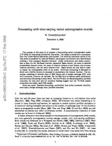
Fig. 1. ME for estimated AR(k ) models from 100 four-dimensional white noise observations as a function of the model order k (1000 simulation runs). Models have been estimated with the NS and LS estimators. The simulation results are accurately described using FST. Also shown are the asymptotic result (Asym) and the exact Cramér–Rao lower bound (CRLB).
VI. FINITE SAMPLE THEORY
(32) with the penalty factor equal to 3 [15]. additional parameters are In vector time series analysis, estimated at once if the model order is increased by 1. Overfit occurs when the reduction of the residual variance is much greater than its expectation due to statistical fluctuations. If the number of additional parameters is large, the fluctuations will become small with respect to the expectation. As a result, the cost of overfit in the case of vector-valued signals is very small. Therefore, the optimal penalty factor is expected to decrease significantly with increasing dimension , approaching the lowest value of as in AIC. V. CRAMÉR–RAO LOWER BOUND FOR THE MODEL ERROR In this section, the exact Cramér–Rao lower bound (CRLB) for the ME of vector AR estimates in normally distributed white is derived. The expression is noise based on the exact likelihood. This means that not only the congiven ditional distribution of the observations is used, but also the distribution of the observations [23]. It can be elementary derived that in white noise the expectation of the ME for an estimator of the VAR( ) model is given by (33) The exact CRLB for the ME is given by [23]
In this section, we will evaluate the finite sample behavior of AR estimators. We will show that this behavior deviates considerably from the asymptotic Taylor approximations and the CRLB. First, we have to establish the maximum model order considered for order selection. The description of the finite sample effects must at least be accurate up to this maximum is equal to the order. The number of estimated parameters for model order . We number of observations will set the maximum model order to half this number, yielding . This is much less restrictive than the maximum mentioned in literature. value To examine the statistical behavior of estimators, AR models vector white noise observations are estimated from with . The results of this simulation experiment are along with the asympgiven in Fig. 1 for dimension totic result and the CRLB. In Fig. 1 the MEs for the NS and LS estimators are given. The simulations show that the error of estimated models is greater than described by the asymptotic Taylor approximation (28). Moreover, the error of the LS estimator is greater than the error of the NS estimator. The framework of FST [17] can be used to describe this behavior of estimators. Also, a finite sample equivalent for the FPE (30) can be derived. The bases of the FST are the finite sample variance coefficients . In scalar time series analysis, represent the variance of the estimated th reflection coefficient. This is generalized to vector signals by using the variance of the estimated partial corabove the true order relation
(34)
(35)
In many cases, actual estimators approach the CRLB. Then, the CRLB is a convenient tool for describing the behavior of estimators. Asymptotically, the CRLB yields the same results as the expressions derived in the previous section. However, the finite behavior of actual estimators deviates considerably from the CRLB, as will be shown in the next section. The lower bound given by equation (34) provides an accurate description for the ME of estimates for low model orders . For higher model orders, the CRLB is very conservative.
are accurately described by the For the two estimators, the following empirical formulae: Nuttall–Strand: Least-Squares: All components
of
(36) are estimated independently.
DE WAELE AND BROERSEN: FINITE SAMPLE EFFECTS IN VECTOR AUTOREGRESSIVE MODELING
921
Using these assumptions, we can derive the finite-sample expression for expectation of the residual (37) A similar expression can be found for the backward residual . Also, we can derive the finite-sample expression above the true order for the expectation for (38) Again, a similar result can be derived for the backward residual . It must be noted that in the derivation of this result the approximation has been used that the stochastic variable can be replaced by . The expectation of the ME in white noise is given by
Fig. 2. Estimates of the PE from 100 observations of a 3-D AR(3)-process compared to the true PE as a function of the model order k (400 simulation runs). The AR models have been estimated with NS. The PE is estimated with FPE and FPE (asymptotic theory) and the FSC.
(39) This expression provides a better description of the actual behavior of the NS estimator than the CRLB (34) or the asymptotic expression (28) (see Fig. 1). It is accurate up to the maximum considered for order selection. The model order deviations for higher order models are caused by the fact that the no longer describe the actual variance of the estimated . As the models that are estimated with the NS algorithm are guaranteed to be stationary, the parameter variance is finite even if the exceeds the total number number of estimated parameters . However, these high-order models have of observations no useful interpretation. With FST, we can accurately describe the difference between the LS and the NS estimators by using different variance coefficients for the two estimators. Combining (37) and (38), we obtain a finite-sample estimator for the PE based on the residual variance, called the finite sample criterion (FSC)
Fig. 3. Experimental eddy-covariance measurements: Simultaneous measurements of the vertical wind velocity w and relative humidity q . The relative humidity is the humidity divided by the air density, yielding a unitless quantity.
(40) The residual covariance RES( ) is calculated from the estimated parameters. This guarantees that the residual variance decreases monotonically. For large , contributions of the order can be neglected. Then, the tend to and FSC tends to FPE. In finite samples, FSC is more accurate than FPE. As a observations of a simulation example, we have used three-dimensional (3-D) AR(3)-process. The average FPE and FSC of 500 simulation runs are given in Fig. 2. The estimate of the PE with FPE or FPE is too low. This explains why the order selected with the AIC tends to be too high. As an example of the application of FST to experimental data, we will use eddy-covariance measurements taken at a sugar-beet field [24]. The dynamics of water evaporation can be derived from the cross correlation of the vertical wind speed with the relative air humidity . The data that have been used for estiobservations mation of AR models are given in Fig. 3 ( per channel). The models have been estimated from these data with the NS and LS estimators. Also, an estimate of the PE is obtained with the FSC as well as the FPE. The quality of the estimators is evaluated by splitting a larger set of data into two
Fig. 4. Estimates of the PE from the experimental eddy-covariance measurements compared to the PE calculated from a set of 3000 new observations. The AR models have been estimated with NS and with LS. The PE for NS is estimated with FPE and the FSC.
segments. The first segment of 300 observations (Fig. 3) is used to estimate the models; the second segment of 3000 observations is used to determine the quality of those models by using them for predicting these observations. In Fig. 4, the PE is given as a function of the model order . As these results are based on a single set of data, obviously they are less accurate than the simulation results which are the average of a large number of simulation runs. Also, practical
922
IEEE TRANSACTIONS ON INSTRUMENTATION AND MEASUREMENT, VOL. 51, NO. 5, OCTOBER 2002
data will never be entirely stationary. Still, the experimental data confirms the conclusions drawn based on the simulations. First, the NS estimator is somewhat more accurate (lower PE) than the LS estimator for higher order models. Second, FSC is a better estimator for PE than FPE. The most important difference is ) as the that FSC is minimal for the same model order ( actual PE as calculated from the new data set. Conversely, FPE ). Also, there is is smallest for very large model orders ( that is lower than the a local minimum in FPE at order . local minimum at VII. EXTENSION TO CHANNEL PREDICTION In channel prediction, the aim is to predict a channel of based on previous observations of the vector . More generally, the aim can be formulated as predicting a linear mapping of , where the dimension of is not necessarily equal to the dimension of . We can use the model estimated for the entire vector and use it to predict . The major differences are found in order selection. The optimal order for prediction of will often be different from the optimal order for prediction of . The finite sample estimate for the PE FSC (40) derived in the previous section can be used without modification. Here, too, the NS algorithm deserves a preference over the LS estimator as it typically has a smaller ME and is guaranteed to provide a stationary model. One application of this algorithm is to provide a robust alternative for the LS ARX estimator for autoregressive models with an exogeneous input (ARX models) in system identification [25]. In this set-up, the vector consists of the input and output of a plant; the channel to be predicted is the output [22]. VIII. CONCLUDING REMARKS Asymptotic theory does not provide an accurate description for the behavior of vector AR estimators for higher model orders. The lower bound for the ME provided by the Cramér–Rao bound is very conservative. Therefore, a FST for vector time series has been developed. With FST an order selection criterion can be formulated with an optimal trade-off of underfit and overfit. It can also be used to find the best model for channel prediction. Investigation of the finite sample behavior of estimators showed that the NS estimator is more robust and generally more accurate than the LS estimator. REFERENCES [1] S. M. Kay and S. L. Marple, “Spectrum analysis—A modern perspective,” Proc. IEEE, vol. 69, pp. 1380–1419, Nov., 1981. [2] H. Akaike and G. Kitagawa, Eds., “The practice of time series analysis,” in Statistics for Engineering and Physical Science. New York: Springer, 1999. [3] K. P. Burnham and D. R. Anderson, Model Selection and Inference. New York: Springer, 1998. [4] P. M. T. Broersen, “Automatic spectral analysis with time series models,” IEEE Trans. Instrum. Meas., vol. 51, pp. 211–216, Apr. 2002. [5] J. Li, G. Liu, and P. Stoica, “Moving target feature extraction for airborne high-range resolution phased-array radar,” IEEE Trans. Signal Processing, vol. 49, pp. 277–289, Feb. 2001. [6] S. L. Marple, Digital Spectral Analysis With Applications. Englewood Cliffs, NJ: Prentice-Hall Signal Processing Series, 1987. [7] M. B. Priestley, Spectral Analysis and Time Series. London, U.K.: Academic, 1981.
[8] C. M. Hurvich and C. L. Tsai, “A corrected Akaike information criterion for vector autoregressive model selection,” J. Time Series Anal., vol. 14, no. 3, pp. 271–279, 1993. [9] T. Subba Rao, Developments in Time Series Analysis. New York: Chapman Hall, 1993, ch. 5, pp. 50–66. [10] H. Akaike, “A new look at statistical model identification,” IEEE Trans. Automat. Contr., vol. AC-19, pp. 716–723, 1974. [11] J. Castro and J. P. LeBlanc, “Model order selection for multidimensional innovations based detection in airborne radar,” in Proc. IEEE Radar Conf., New York, 1998, pp. 141–146. [12] S. M. Kay, Modern Spectral Estimation. Englewood Cliffs, NJ: Prentice-Hall, 1988. [13] Y. Sakamoto, M. Ishiguro, and G. Kitagawa, Akaike Information Criterion Statistics. Tokyo, Japan: KTK Scientific, 1986. [14] J. R. Roman, M. Rangaswamy, D. W. Davis, Q. Zhang, B. Himed, and J. H. Michels, “Parametric adaptive matched filter for airborne radar applications,” IEEE Trans. Aerospace Electron. Syst., vol. 36, pp. 677–691, Apr. 2000. [15] P. M. T. Broersen and H. E. Wensink, “On the penalty factor for autoregressive order selection in finite samples,” IEEE Trans. Signal Processing, vol. 44, pp. 748–752, Mar. 1996. [16] K. Holden, “Vector autoregression modeling and forecasting,” J. Forecasting, vol. 14, no. 3, pp. 159–166, 1995. [17] P. M. T. Broersen, “Finite sample criteria for autoregressive order selection,” IEEE Trans. Signal Processing, vol. 48, pp. 3550–3558, Dec. 2000. [18] W. Greub, “Linear algebra,” in Graduate Texts in Mathematics, 4th ed. New York: Springer, 1981. [19] G. H. Golub and C. F. Van Loan, Matrix Computations, 2nd ed. Baltimore, MD: John Hopkins Univ. Press, 1989. [20] P. J. Brockwell and R. A. Davis, Time Series: Theory and Methods. New York: Springer-Verlag, 1990. [21] J. Durbin, “The fitting of time series models,” Rev. Inst. Int. Stat., vol. 28, pp. 233–243, 1960. [22] H. Akaike, “Autoregressive model fitting for control,” Ann. Inst. Stat. Math., vol. 23, pp. 163–180, 1971. [23] S. de Waele and P. M. T. Broersen, “Finite sample effects in multichannel autoregressive modeling,” in Proc. IMTC Conf., Budapest, Hungary, 2001, pp. 1–6. [24] W. M. L. Meijninger, O. K. Hartogensis, W. Kohsiek, J. C. B. Hoedjes, R. M. Zuurbier, and H. A. R. De Bruin, “Determination of area averaged sensible heat fluxes with a large aperture scintillometer over a heterogeneous surface—Flevoland field experiment,” Boundary-Layer Meteorol., 2002, to be published. [25] L. Ljung, System Identification-Theory for the User, second ed. Upper Saddle River, NJ: Prentice Hall, 1999.
Stijn de Waele was born in Eindhoven, The Netherlands, in 1973. He received the M.Sc. degree in applied physics in 1998 from Delft University of Technology, Delft, The Netherlands, where he is currently pursuing the Ph.D. degree in the Department of Applied Physics. His research interests are the development of new time series analysis algorithms and its application to radar signal processing.
Piet M. T. Broersen was born in Zijdewind, The Netherlands, in 1944. He received the M.Sc. degree in applied physics in 1968 and the Ph.D. degree in 1976, both from the Delft University of Technology, Delft, The Netherlands. He is currently with the Department of Applied Physics of the Delft University. His main research interest is automatic identification. He found a solution for the selection of order and type of time series models and the application to spectral analysis, model building, and feature extraction. The next subject is the automatic identification of input–output relations with statistical criteria.