Fitting of NWM Ray-tracing to Closed-form Tropospheric Model Expressions
Landon Urquhart1, Felipe Nievinski2 and Marcelo Santos1 1. Department of Geodesy and Geomatics Engineering, University of New Brunswick 2. Department of Aerospace Engineering Sciences, University of Colorado, Boulder, CO
1
Outline Objectives and Goals Development of Mapping Functions
Experiment Evaluation and Results ▪ Symmetric Mapping Functions ▪ Asymmetric Mapping Functions Conclusion and Future Work
2
Objectives and Goals Ray-tracing is a promising technique for describing the elevation- and azimuth- dependence of the tropospheric delay, but:
1) very time consuming 2) difficult to distribute to end users OBJECTIVE Develop closed-form mapping functions which can sufficiently model the full information contained within the Numeric Weather Model, including the asymmetric nature of the atmosphere REQUIRED Evaluate the mathematical models used for tropospheric delay modelling. 3
Development of MFs Mathematical Model Describes how the delay varies with respect to some parameter Ex. mf ( )
1 sin
a sin ...
Realization Through Ray-tracing Mapping Functions Obtained by fitting mathematical model to ray-traced observations
Ray-tracing Various atmospheric sources and structures 4
Mapping Functions L(e, ) Lz mfsym (e) mfasym (e, ) Fasym ( ) mfsym (e) cot(e) Symmetric Mathematical Models
Gradient Functions
Marini, J.W. (1972). Radio Science, Vol. 7, No 2, pp.223-231.
Davis, J.L. et al. (1993). Radio Science, Vol. 28, No 6, pp 1003-1018
Yan and Ping (1995). The Astronomical Journal, Vol. 110, No. 2, pp 934-939
Seko et al., (2004) J. Meteorolgical Society of Japan Vol. 82, pp. 339--350,
Boehm et al. (2006). J. Geophys. Res., vol 111, B02406
Boehm, J., and H. Schuh (2001). 5
Experiment Evaluate site-specific mapping functions using ray-traced observations from 3D NWM. Fitting data: Azimuths: 0, 90, 180, 270 Elev. Angle: 3, 4, 6, 8, 14, 30, 70
Canadian Regional NWM ▪15 km Horizontal resolution ▪28 isobaric levels + sfc level 0
Experiment Location:
1500
Northing (km)
Truth data: Elev. Angle: 3, 5, 7, 10 Azimuth: Every 15 degrees
Station: CAGS Gatineau, Quebec Epochs: 00:00h every 5th day of 2008
3000
4500
-2000
-1000
0
1000 2000 Easting (km)
3000
4000
6
Results: Symmetric MF Residuals by Elevation Angle Non hydro.
10
20
Mean (mm)
Marini 3 coefficients
Mean (mm)
Hydro. + geom.
0
-10
3
4
6
-20
8 14 30 70
0
-10
3
4
6
8 14 30 70
-20
Mean (mm)
Mean (mm)
6
8 14 30 70
3
4
6
8 14 30 70
3
4
6
8 14 30 70
20
0
-10
4
0
10
Yan and Ping
3
20
Mean (mm)
Mean (mm)
10
Marini 4 coefficients
0
3
4
6
8 14 30 70
0
-20
Elevation Angle (degrees)
Error Bars shown in cm for convenience!!
7
Results: Symmetric MF bias (mm)
40 20 0 -20
3
5
7
10
5 bias (mm)
Non-Hydro.
Hydrostatic
Truth minus mapped, by Elevation Angle
0
Yan & Ping 50 3 coeff. Marini 0 4 coeff. Marini -50 mVMF 35710
-5 -10
3
5 7 Elevation Angle (degrees)
10 8
Results: Symmetric MF Difference in delay (00:00h) December 31st, 2008 Delay (Metres)
60 Marini 4 Coeff. 100 UNSW 50 0 mVMF 0 50 Marini 3 Coeff.
40 20 0 0
10
20 30 40 Elevation Angle (degrees)
50
Difference (mm)
Difference with respect to Marini 3 Coeff. 10 0 Marini 4 Coeff. 10 0 UNSW -10 310 71525 mVMF
-10 3
7
10
15 25 Elevation Angle (degrees)
Nominal zenith delay of 2300 mm used!!
9
Results: Symmetric MF Descrepancy (mm)
Descrepancy (mm)
Non-Hydro.
Hydrostatic
Discrepancy at 5o elevation angle 200 0 -200 0
500
1000 observation #
1500
1000 observation #
1500
Yan & Ping 1000 Marini 3 Coeff. 0 -1000 Marini 4 coeff. 01000 2000 mVMF
1000 0 -1000 0
500
2000
2000
10
Results: Asymmetric MF Residuals by Elevation Angle
Non hydro.
2nd Order Polynomial
-5 5
3
4
6
8 14 30 70
0 -5
3
4
6
8 14 30 70
5 0 -5 5
3
4
6
8 14 30 70
0 -5
3
4
6
8 14 30 70
Mean (mm) Mean (mm)
0
Mean (mm)
5
Mean (mm)
Spherical Harmonics (m=2,n=1)
Mean (mm)
Spherical Harmonics (m=1,n=1)
Mean (mm)
Linear Gradient Model
Mean (mm) Mean (mm)
Hydro. + geom. 5 0 -5 0
3
4
6
8 14 30 70
3
4
6
8 14 30 70
3
4
6
8 14 30 70
3
4
6
8 14 30 70
-200 -400 5 0 -5 5 0 -5
Elevation Angle (degrees)
Error Bars shown in cm for convenience!!
11
Results: Asymmetric MF Truth minus mapped, sorted by Elevation Angle bias (mm)
5 0 -5
3
5 7 Elevation Angle (degrees)
1000 bias (mm)
Non-Hydro.
Hydrostatic
10
10 2nd Order Poly. 1000 SH11 0 SH21 -1000 0 5Gradient 10 Model Standard
500 0 -500 2
4 6 8 Elevation Angle (degrees)
10 12
Results: Asymmetric MF
Descrepancy (mm)
Non-Hydro.
Hydrostatic
Descrepancy (mm)
Discrepancy at 5o elevation angle 50 0 -50 500
1000 observation #
1500
500
1000 observation #
1500
500
2nd 2000 Order Poly. SH11 0 -2000 Standard01000 Gradient 2000 Model SH21
0 -500 -1000
13
Conclusions Differences between Yan and Ping (1995) and Marini (1972) are several mm’s when derived from same atm. source Spherical harmonics seem promising: Hydrostatic appears excellent but work needs to be done on non-hydrostatic modelling One option is to look at gradient mapping functions such as that suggested by Chen and Herring (1997). Additionally, splines or polynomials. Must expand experiment locations to get a variety of atmospheric conditions. 14
References Boehm, J., B. Werl, and H. Schuh (2006), “Troposphere mapping functions for GPS and very long baseline interferometry from European Centre for Medium-Range Weather Forecasts operational analysis data”, J. Geophys. Res., Vol. 111. Bohm, J., and H. Schuh (2001). “Spherical harmonics as a supplement to global tropospheric mapping functions and horizontal gradients.” Proceedings of the 15th Working Meeting on European VLBI for Geodesy and Astrometry, September 7–8, pp. 143148. Davis, J. L., G. Elgered, A. E. Niell, and C. E. Kuehn (1993). “Ground-based measurementof gradients in the “wet” radio refractivity of air.” Radio Science, Vol. 28, No. 6, pp.1003– 1018. Marini, J. W. (1972). “Correction of satellite tracking data for an arbitrary tropospheric profile.” Radio Science, Vol. 7, No. 2, pp. 223–231. Seko, H., H. Nakamura, and S. Shimada (2004). “An evaluation of atmospheric models for GPS data retrieval by output from a numerical weather model.” Journal of the Meteorological Society of Japan, Vol. 82, No. 1B, pp. 339–350. Yan, H., and J. Ping (1995). “The generator function method of the tropospheric refraction corrections.” The Astronomical Journal, Vol. 110, No. 2, pp. 934–939. 15
16
Santos, 2004
[email protected]