Formal Verification based on Boolean Expression ...

Electronic Notes in Theoretical Computer Science 56 (2001) http://www.elsevier.nl/locate/entcs/volume56.html 190 pages

Formal Veri cation based on Boolean Expression Diagrams Poul Frederick Williams

c 2001 Published by Elsevier Science B. V.

Abstract This dissertation examines the use of a new data structure called Boolean Expression Diagrams (BEDs) in the area of formal veri cation. The recently developed data structure allows fast and eÆcient manipulation of Boolean formulae. Many problems in formal veri cation can be cast as problems on Boolean formulae. We chose a number of such problems and show how to solve them using BEDs. Equivalence checking of combinational circuits is a formal veri cation problem which translates into tautology checking of Boolean formulae. Using BEDs we are able to preserve much of the structure of the circuits within the Boolean formulae. We show how to exploit the structural information in the veri cation process. Sometimes combinational circuits are speci ed in a hierarchical or modular way. We present a method for verifying equivalence between two such circuits. The method builds on cut propagation. Assuming that the two circuits are given identical inputs, we propagate this knowledge through the circuits from the inputs to the outputs. The result is the knowledge of how the outputs of the two circuits correspond, e.g., are the outputs of the two circuits pairwise equivalent? The circuits and the movements of cuts can be described using Boolean formulae. Symbolic model checking is a technique for verifying temporal speci cations of nite state machines. It is well known how nite state machines and the evaluation of the temporal speci cations can be expressed using Boolean formulae. We show how to do these manipulations using BEDs. We concentrate on examples which are hard for standard symbolic model checking methods. Determining whether a formula is satis ability is a problem which occurs in veri cation of combinational circuits and in symbolic model checking. Often satis ability checking is associated with detecting errors. We examine how satis ability checking can be done using the BED data structure. Finally, we take a look at how it is possible to extend the BED data iii

iv structure. Among other operations, we introduce an operator for computing minimal p-cuts in fault trees. A fault tree is a Boolean formula expressing whether a system fails based on the condition (\failure" or \working") of each of the components. A minimal p-cut is a representation of the most likely reasons for system failure. This method can be used to calculate approximately the probability of system failure given the failure probabilities of each of the components. As part of this research, we have developed a BED package. The appendix describes the package from a user's point of view. Note Added in Print This book is a slight revision of the author's Ph.D. thesis [Wil00].

Acknowledgements I would like to thank my two supervisors at the Technical University of Denmark (now both with the IT University of Copenhagen), Associate Professors Henrik Reif Andersen and Henrik Hulgaard, for giving me the opportunity to work on this project. During my graduate studies, they have guided me, given me valuable comments and criticism on my work, and patiently answered my many questions. For this I am them grateful. A special thanks is due to Professor Edmund Clarke from Carnegie Mellon University. I spent six months working with him and his model checking group in Pittsburgh. His vast knowledge of computer science and the inspiring atmosphere surrounding him and his group made it a joy to work with him. Thanks are also due to Charge de Recherches Antoine Rauzy from Centre National de la Recherche Scienti que, Associate Professor David Sherman and Assistant Professor Macha Nikolskaa from Universite Bordeaux I. During David and Macha's visit to Lyngby and my subsequent visit to Bordeaux, we worked together and became friends in the process. During my research, I have had long and fruitful discussions with fellow doctoral students. Especially Jrn Lind-Nielsen from Technical University of Denmark and Anubhav Gupta from Carnegie Mellon University have lent an ear, made helpful suggestions, and answered my numerous questions. Rune Mller Jensen, Ken Friis Larsen, Jakob Lichtenberg, Jesper Mller and many others have also been helpful. I am indebted to the members of my Ph.D. committee: Associate Professor Hans Henrik Lvengreen from Technical University of Denmark, Professor Parosh Abdulla from Chalmers University, and Nils Klarlund from AT&T in New Jersey. Thank you for valuable comments and criticism on my thesis.

v

Contents List of Algorithms and Figures

xi

List of Tables

xiii

Symbols

xv

1 Introduction

1.1 1.2 1.3 1.4 1.5

Formal Veri cation . . . . Logic . . . . . . . . . . . . Aim of This Dissertation . Safety and Reliability . . Overview . . . . . . . . .

. . . . .

. . . . .

.. .. .. .. ..

. . . . .

.. .. .. .. ..

. . . . .

. . . . .

.. .. .. .. ..

. . . . .

.. .. .. .. ..

. . . . .

.. .. .. .. ..

. . . . .

. . . . .

. . . . .

. . . .

.. .. .. ..

. . . .

.. .. .. ..

. . . .

. . . .

.. .. .. ..

. . . .

.. .. .. ..

. . . .

.. .. .. ..

. . . .

. . . .

. . . .

3.1 Introduction . . . . . . . . . . . . . . . . . . . . . . 3.2 Simpli cations . . . . . . . . . . . . . . . . . . . . 3.2.1 Operator Sets . . . . . . . . . . . . . . . . . 3.2.2 Rewriting . . . . . . . . . . . . . . . . . . . 3.2.3 Other Simpli cation Methods . . . . . . . . 3.2.4 Experimental Results for Simpli cations . . 3.3 Variable Ordering . . . . . . . . . . . . . . . . . . . 3.3.1 The Fanin Heuristic . . . . . . . . . . . . . 3.3.2 The Depth Fanout Heuristic . . . . . . . 3.4 Stalmarck's Method . . . . . . . . . . . . . . . . .

. . . . . . . . . .

.. .. .. .. .. .. .. .. .. ..

. . . . . . . . . .

. . . . . . . . . .

. . . . . . . . . .

2 Boolean Expression Diagrams

2.1 2.2 2.3 2.4

Data Structure Properties . . . Algorithms . . Related Work .

. . . .

.. .. .. ..

. . . .

.. .. .. ..

. . . .

3 Flat Equivalence Checking

vii

1

3 4 6 8 9

13

13 18 20 28

33

33 36 36 37 41 43 45 48 49 50

viii 3.4.1 Implementation of Stalmarck's Method using BEDs 3.5 Experimental Results . . . . . . . . . . . . . . . . . . . . . . 3.5.1 The ISCAS'85 Benchmark Suite . . . . . . . . . . . 3.5.2 The LGSynth'91 Benchmark Suite . . . . . . . . . . 3.5.3 Stalmarck's Method . . . . . . . . . . . . . . . . . . 3.6 Related Work . . . . . . . . . . . . . . . . . . . . . . . . . . 3.7 Conclusion . . . . . . . . . . . . . . . . . . . . . . . . . . . 4 Hierarchical Equivalence Checking

4.1 Introduction . . . . . . . . . . . . . . . 4.2 Hierarchical Combinational Circuits . 4.3 Cut Propagation . . . . . . . . . . . . 4.3.1 Example . . . . . . . . . . . . . 4.3.2 Moving Cuts . . . . . . . . . . 4.3.3 Build vs. Propagate . . . . . . 4.4 Experimental Results . . . . . . . . . . 4.5 Related Work . . . . . . . . . . . . . . 4.6 Conclusion . . . . . . . . . . . . . . .

.. .. .. .. .. .. .. .. ..

. . . . . . . . .

.. .. .. .. .. .. .. .. ..

. . . . . . . . .

. . . . . . . . .

. . . . . . . . .

5.1 Introduction . . . . . . . . . . . . . . . . . . . . . . 5.2 Theory of Model Checking . . . . . . . . . . . . . . 5.2.1 Computation Tree Logic . . . . . . . . . . . 5.2.2 Model Checking using Propositional Logic . 5.3 Model Checking with BEDs . . . . . . . . . . . . . 5.3.1 Quanti cation . . . . . . . . . . . . . . . . 5.3.2 Satis ability Checking . . . . . . . . . . . . 5.3.3 Example . . . . . . . . . . . . . . . . . . . . 5.4 Experimental Results . . . . . . . . . . . . . . . . . 5.4.1 Multiplier . . . . . . . . . . . . . . . . . . . 5.4.2 Barrel Shifter . . . . . . . . . . . . . . . . . 5.5 Model Checking of lfp-CTL . . . . . . . . . . . . . 5.5.1 Theory . . . . . . . . . . . . . . . . . . . . 5.5.2 Implementation . . . . . . . . . . . . . . . . 5.6 Related Work . . . . . . . . . . . . . . . . . . . . . 5.7 Conclusion . . . . . . . . . . . . . . . . . . . . . .

. . . . . . . . . . . . . . . .

.. .. .. .. .. .. .. .. .. .. .. .. .. .. .. ..

. . . . . . . . . . . . . . . .

. . . . . . . . . . . . . . . .

. . . . . . . . . . . . . . . .

5 Symbolic Model Checking

6 Satis ability

. . . . . . . . .

. . . . . . . . .

.. .. .. .. .. .. .. .. ..

. . . . . . . . .

. . . . . . .

55 57 57 63 66 72 75 77

77 79 82 82 84 86 87 89 89

91

91 93 95 99 101 103 108 110 114 115 118 120 121 126 127 129 131

6.1 Introduction . . . . . . . . . . . . . . . . . . . . . . . . . . . . 131 6.2 Satis ability Using CNF Formulae . . . . . . . . . . . . . . . 132

ix 6.3 6.4 6.5 6.6

Satis ability Using BEDs Experimental Results . . . Related Work . . . . . . . Conclusion . . . . . . . .

.. .. .. ..

. . . .

. . . .

.. .. .. ..

. . . .

.. .. .. ..

. . . .

.. .. .. ..

. . . .

. . . .

. . . .

7.1 Introduction . . . . . . . . . . . . . . . 7.2 New Types of Vertices . . . . . . . . . 7.2.1 Existential Quanti cation . . . 7.2.2 Universal Quanti cation . . . . 7.2.3 Substitution . . . . . . . . . . . 7.2.4 Operators on Vectors . . . . . . 7.2.5 Implementation . . . . . . . . . 7.3 Fault Tree Analysis . . . . . . . . . . . 7.3.1 Minimal P-Cuts with BEDs . . 7.4 Experimental Results . . . . . . . . . . 7.4.1 Substitution . . . . . . . . . . . 7.4.2 P-Cut . . . . . . . . . . . . . . 7.5 Related Work . . . . . . . . . . . . . . 7.6 Conclusion . . . . . . . . . . . . . . .

. . . . . . . . . . . . . .

. . . . . . . . . . . . . .

.. .. .. .. .. .. .. .. .. .. .. .. .. ..

. . . . . . . . . . . . . .

.. .. .. .. .. .. .. .. .. .. .. .. .. ..

. . . . . . . . . . . . . .

.. .. .. .. .. .. .. .. .. .. .. .. .. ..

. . . . . . . . . . . . . .

. . . . . . . . . . . . . .

. . . . . . . . . . . . . .

7 Extending BEDs

. . . .

. . . .

.. .. .. ..

. . . .

133 135 138 138 141

141 142 142 143 144 145 150 151 154 156 156 157 159 160

8 Conclusion

161

A The BED Tool

165

Bibliography

177

Index

189

8.1 Future Directions . . . . . . . . . . . . . . . . . . . . . . . . . 163

List of Algorithms and Figures 1.1 1.2 2.1 2.2 2.3 2.4 2.5 2.6 2.7 2.8 2.9 2.10 3.1 3.2 3.3 3.4 3.5 3.6 3.7 3.8 3.9 3.10 3.11 3.12 3.13 3.14

Two equivalent combinational circuits . . . . . . . . . . The real and the formal worlds . . . . . . . . . . . . . . An example of a BED . . . . . . . . . . . . . . . . . . . The BED array . . . . . . . . . . . . . . . . . . . . . . . The Mk algorithm . . . . . . . . . . . . . . . . . . . . . Memory usage in BDD construction . . . . . . . . . . . The up step . . . . . . . . . . . . . . . . . . . . . . . . . The Up One algorithm . . . . . . . . . . . . . . . . . . The Up One0 algorithm . . . . . . . . . . . . . . . . . . The Apply algorithm . . . . . . . . . . . . . . . . . . . The Up All algorithm . . . . . . . . . . . . . . . . . . The Up algorithm . . . . . . . . . . . . . . . . . . . . . Circuit with memory . . . . . . . . . . . . . . . . . . . . Rewrite rules for BEDs . . . . . . . . . . . . . . . . . . The Mk algorithm (modi ed for rewriting rules) . . . . Lost sharing . . . . . . . . . . . . . . . . . . . . . . . . . Balancing BEDs . . . . . . . . . . . . . . . . . . . . . . The 17th output bit of multipliers . . . . . . . . . . . . The 17th output bit of multipliers with rewriting rules . A four-input AND gate and a corresponding BED . . . The Fanin heuristic . . . . . . . . . . . . . . . . . . . . The Depth Fanout heuristic . . . . . . . . . . . . . . Parse-tree for Boolean formulae . . . . . . . . . . . . . . Rules A for the triplet u $ l ^ h. . . . . . . . . . . . . The 0-Sat algorithm . . . . . . . . . . . . . . . . . . . . The (k + 1)-Sat algorithm . . . . . . . . . . . . . . . . . u

xi

. . . . . . . . . . . . . . . . . . . . . . . . . .

. . . . . . . . . . . . . . . . . . . . . . . . . .

. . . . . . . . . . . . . . . . . . . . . . . . . .

1 3 17 18 19 21 22 24 25 26 27 29 34 39 40 41 42 46 47 48 49 50 51 52 53 53

xii 3.15 3.16 4.1 4.2 4.3 4.4 4.5 4.6 5.1 5.2 5.3 5.4 5.5 5.6 5.7 5.8 5.9 5.10 6.1 6.2 6.3 7.1 7.2 7.3 7.4 7.5 7.6 7.7 7.8

Parse-tree for 0-hard Boolean formulae . . . . . . . . . . A 1-hard and a 0-easy BED . . . . . . . . . . . . . . . . Hierarchical 4-bit adder . . . . . . . . . . . . . . . . . . Two 4-bit adders . . . . . . . . . . . . . . . . . . . . . . The Prop algorithm . . . . . . . . . . . . . . . . . . . . The Build algorithm . . . . . . . . . . . . . . . . . . . The Propagate algorithm . . . . . . . . . . . . . . . . Two hierarchical circuits . . . . . . . . . . . . . . . . . . An SMV program and the associated Kripke structure . A modi ed Kripke structure . . . . . . . . . . . . . . . . The Lfp and Gfp operators . . . . . . . . . . . . . . . . The QbS algorithm . . . . . . . . . . . . . . . . . . . . The EF algorithm . . . . . . . . . . . . . . . . . . . . . A modulo-4 counter . . . . . . . . . . . . . . . . . . . . SMV program for a modulo-4 counter . . . . . . . . . . BEDs for transition function . . . . . . . . . . . . . . . Graph of runtimes for multiplier example . . . . . . . . The ModelCheck algorithm . . . . . . . . . . . . . . . The DP (Davis-Putnam) algorithm . . . . . . . . . . . . The BedSat algorithm . . . . . . . . . . . . . . . . . . An illustration of the BedSat algorithm . . . . . . . . . Vector existential quanti cation . . . . . . . . . . . . . . The up step for map vertices . . . . . . . . . . . . . . . The Mk algorithm modi ed for ESUB . . . . . . . . . . The Up One0 algorithm modi ed for ESUB . . . . . . . The Up All algorithm modi ed for ESUB . . . . . . . Illustration of p-cut computation . . . . . . . . . . . . . A 2n-bit multiplier . . . . . . . . . . . . . . . . . . . . . A 2n-bit multiplier using substitution . . . . . . . . . .

. . . . . . . . . . . . . . . . . . . . . . . . . . . . .

. . . . . . . . . . . . . . . . . . . . . . . . . . . . .

. . . . . . . . . . . . . . . . . . . . . . . . . . . . .

55 56 78 79 84 85 85 87 93 94 97 104 106 110 111 112 117 126 133 134 136 147 148 150 151 152 156 157 158

List of Tables 2.1 2.2 2.3 3.1 3.2 3.3 3.4 3.5 3.6 3.7 3.8 3.9 3.10 3.11 3.12 3.13 3.14 3.15 4.1 5.1 5.2 5.3 5.4 5.5 5.6 6.1 6.2

The 16 binary Boolean connectives and their truth tables . Overview of decision diagrams . . . . . . . . . . . . . . . . . References to decision diagrams . . . . . . . . . . . . . . . . ISCAS'85 results without simpli cations . . . . . . . . . . . ISCAS'85 results with simpli cations . . . . . . . . . . . . . Size and functionality of the ISCAS'85 benchmark circuits . Erroneous circuits from the ISCAS'85 benchmark suite . . . ISCAS'85 results for Up All . . . . . . . . . . . . . . . . . ISCAS'85 results for Up One . . . . . . . . . . . . . . . . . ISCAS'85 comparisons I . . . . . . . . . . . . . . . . . . . . ISCAS'85 comparisons II . . . . . . . . . . . . . . . . . . . Combinational LGSynth'91 circuits (easy) . . . . . . . . . . Combinational LGSynth'91 circuits (hard) . . . . . . . . . . Sequential LGSynth'91 circuits (easy) . . . . . . . . . . . . Sequential LGSynth'91 circuits (hard) . . . . . . . . . . . . Boolean satis ability test cases . . . . . . . . . . . . . . . . ISCAS'85 results for Stalmarck's method . . . . . . . . . . . The eect of minimizing . . . . . . . . . . . . . . . . . . . . Hierarchical adders and multipliers . . . . . . . . . . . . . . Correspondence between set and logic notations . . . . . . . 16-bit multipliers . . . . . . . . . . . . . . . . . . . . . . . . Iterative squaring . . . . . . . . . . . . . . . . . . . . . . . . Bug D . . . . . . . . . . . . . . . . . . . . . . . . . . . . . . Large shift-and-add multipliers . . . . . . . . . . . . . . . . Barrel shifters . . . . . . . . . . . . . . . . . . . . . . . . . . Satis ability and tautology . . . . . . . . . . . . . . . . . . BedSat on ISCAS'85 benchmarks . . . . . . . . . . . . . . xiii

. . . . . . . . . . . . . . . . . . . . . . . . . . .

15 31 32 44 44 58 59 60 61 63 64 67 68 69 70 71 71 72 88 100 116 118 119 120 121 132 137

xiv 6.3 BedSat on model checking problems . . . . . . . . . . . . . . 139 7.1 Veri cation of large integer multipliers . . . . . . . . . . . . . 158 7.2 P-cut results on industrial examples . . . . . . . . . . . . . . 159

Symbols The following notation is used throughout this dissertation: Notation Description

Reference LOGIC

0 1

a, b, c x, y ;  f , g, h [=x]

:

K0

^ 6 ! 6

1 2

False True Boolean variables Boolean variables or vectors of Boolean variables Formulae Formulae Substitution of formula  for variable x in  Negation Connective, constant 0 Connective, conjunction Connective, negated implication Connective, projection on rst argument Connective, negated left-implication Connective, projection on second argument

Table 2.1 Table 2.1 Table 2.1 Table 2.1 Table 2.1 Table 2.1

(continued on next page)

xv

xvi Notation  _ _ $

2 1

! ^

K1 x ! ; 

9 8

(
) TAUT(
)  SAT

S

Description Connective, exclusive or Connective, disjunction Connective, negated disjunction Connective, biimplication Connective, negation of second argument Connective, left-implication Connective, negation of rst argument Connective, implication Connective, negated conjunction Connective, constant 1 If-then-else operator Any binary Boolean connective Existential quanti cation Universal quanti cation Satis ability problem Tautology problem Characteristic function for set S

Reference Table 2.1 Table 2.1 Table 2.1 Table 2.1 Table 2.1 Table 2.1 Table 2.1 Table 2.1 Table 2.1 Table 2.1 Equation 2.1 De nition 1.2.2 De nition 1.2.3 De nition 1.2.5

BED 0 1 u, v, l, h low (v), high (v) var (v), op (v)  f sup (v) v

Zero terminal One terminal Vertices Low and high attributes of vertex Variable and operator attributes of vertex Either a variable or an operator. (v) is short for either var (v) or op (v). Boolean function de ned by vertex Support of BED

Section 2.1 Section 2.1 De nition 2.1.1 De nition 2.1.1 De nition 2.1.2 De nition 2.1.5

(continued on next page)

xvii

Symbols

Notation Description jvj Size of BED BED for  The BED obtained by a straightforward translation of formula  BED u The BED rooted at vertex u Ordering of variables or vertices < depth(v) The depth of a vertex v Path from vertex u to vertex v u v

Reference De nition 2.1.6 De nition 2.1.8 Section 2.1 De nition 3.3.1 De nition 2.1.7

STALMARCK , R k

C A

u

Equivalence relation Saturation depth Set of axioms from equivalence relation  Set of rules from vertex (triplet) u

Section 3.4 Section 3.4 Equation 3.2 Section 3.4

HIERARCHICAL CIRCUITS HCC (C; c) c i s,t,u,v,x,y p K H R R [Map] in

out

Hierarchical combinational circuit. It consists of a set of cells C and a top cell c 2 C . Cell Instantiation of a cell Variables or vectors of variables Path in a container cell Cut Cut-relation Input relation Output relation Renaming of variables

De nition 4.2.1 De nition 4.2.2 De nition 4.2.3 De nition 4.2.4 De nition 4.2.5 De nition 4.2.6 Equation 4.2 (Equation 4.2)

(continued on next page)

xviii Notation Description M T I X S s x `

A

s

s M i

s

x

i

j

s j=  [ ] [ ] k

k

[]

k

=  s

j

Reference

MODEL CHECKING

Finite state machine Transition function / relation Set of initial states Set of inputs Set of states State Input Labeling of states Set of atomic propositions Transition from state s to state s on input

De nition 5.2.2 De nitions 5.2.1 and 5.2.2 De nition 5.2.2 De nition 5.2.2 De nition 5.2.2

Path of length k from state s to state s System M models speci cation  Semantics of CTL formula  Similar to [ ] but with exactly k iterations in each xed point computation Similar to [ ] but with input variables still in the formulae CTL formulae  and  are s-equivalent

De nition 5.2.4 De nitions 5.2.5 and 5.2.14 De nition 5.2.10 De nition 5.5.4

i

j

x

i

j

k

De nition 5.2.2 De nition 5.2.2 De nition 5.2.3

De nition 5.5.7 De nition 5.5.9

FAULT TREES x L; X x:L   c

X

Boolean variable Sets of variables Union of sets fxg and L Product of only positive literals Minterm for formula f obtained by adding to  the negative literals formed over all the variables in f but not 

Section 7.3 Section 7.3 Section 7.3 Section 7.3 Section 7.3 (continued on next page)

xix

Symbols

Notation Description Reference (f ) Set of minimal p-cuts for f Section 7.3  (f ) Set of minimal p-cuts for f with at most k Section 7.3 literals in length k

MISCELLANEOUS B R Z

7! P (
) 

The set f0; 1g The set of all real numbers The set of all integers Mapping Assignment Power set Set transformer

De nition 5.2.7

Chapter 1

Introduction Once I gave a seminar at a company about my research. I presented the combinational circuits in Figure 1.1, and asked the question whether the two circuits were equivalent? I demonstrated my formal veri cation technique 1

i1

i1

o01

i2 i3

i3

o02

i4

o001

i2 i4

o002

: Two equivalent combinational circuits.

Figure 1.1

by proving that output o0 and output o00 are equivalent. After the seminar a couple of people from the audience came to me and said that the second pair of outputs were not equivalent. They argued that output o0 only depends on inputs i and i , while output o00 depends on i , i , and i . Their argument is correct. However, a more careful analysis of output o00 shows that the value of input i is masked by the circuitry and therefore cannot in uence the value of the output. Thus the two circuits are indeed equivalent. Stories like this one show that human reasoning is prone to errors. We cannot always rely on our intuition. We need a systematic way of handling these tasks such that we know for sure that we have covered all possibilities and left nothing out. Another complicating factor is the complexity of the problems we want 1

1

2

3

4

2

2

3

4

2

2

1 For the purpose of simplicity, we chose to ignore transients, glitches, and other real-life phenomena in circuits.

1

2

CHAPTER 1. INTRODUCTION

to solve. Again the equivalence checking problem is a good example. Each input can be either high or low. With four inputs, we have 2 = 16 input combinations, which is no big deal as we can just handle each combination by itself. A larger circuit may have a hundred inputs. This leads to 2 = 1; 267; 650; 600; 228; 229; 401; 496; 703; 205; 376 input combinations. Or more than a thousand billion billion billion combinations. Such a large number of combinations cannot be handled one by one. If we cannot try all the input combinations to see if they result in the expected behavior for our system, how can we be certain that there are no errors? One of the untested input combinations may provoke an erroneous behavior of the system. But if we do not try that input combination, we never nd the error. Mathematicians have solved similar problems for centuries. Consider the mathematical theorem which says that for real numbers, multiplication distributes over addition: a
(b + c) = a
b + a
c : The variables a, b and c are abstractions of real numbers. Mathematicians have proven that for any value of the three variables, the above equation holds. Nobody would, or could, try all the in nitely many possible values of a, b and c. In much the same way we can recognize structure in the systems we deal with. For example, we may recognize that one input i of the 100 inputs to a circuit is only used if another input j is high. Otherwise i is ignored. There is therefore no need to consider input combinations which dier only in i when j is low. Given, for example, the two combinational circuits in Figure 1.1, how do we proceed with proving that they are equivalent? What should our overall strategy be? Consider Figure 1.2. It shows the real and the formal worlds. Given a real world problem, we want to nd a real world solution. This is indicated by edge 1. However, in practice it is hard to solve problems in the real world. A possibility is to formalize the problem (edge 2). A formal problem is one described in mathematics and logic. Staying in the formal world, we can solve the formal problem (edge 3), and transform the formal solution back to a real solution (edge 4). The route 2-3-4 might seem as a detour over just taking edge 1. But going via the formal world, we can reason about our methods, and we have a set of mathematical and logical tools available. In this dissertation we stay exclusively in the formal world. We assume that the transitions between the two worlds (edges 2 and 4) are either triv4

100

3

1.1. FORMAL VERIFICATION (1) Real problem

Real solution

(2)

(4)

(3) Formal problem

Formal solution

Figure 1.2: The real and the formal worlds illustrated by the two circles. The edges indicate how to solve a real world problem by either staying in the real world (edge 1) or going via the formal world (edges 2, 3, and 4).

ially simple or that someone else takes care of them. This does not mean that those transitions are uninteresting. On the contrary, they are very interesting. The whole idea of how to formalize a problem, including deciding which parts to abstract away and which parts to model, is a major research area these days. 1.1 Formal Veri cation The title of this dissertation is \Formal Veri cation Based on Boolean Expression Diagrams". In this section we de ne what we mean by formal veri cation. According to Merriam-Webster's dictionary , the word \veri cation" means \the act or process of verifying" and \to verify" means \to establish the truth, accuracy, or reality of." The word \formal" means \relating to or involving the outward form, structure, relationships, or arrangement of elements rather than content." So formal veri cation is the process of establishing the truth using outward form, structure, relationships, or arrangement of elements rather than content. To get a workable de nition of formal veri cation, we propose \the act of proving whether a system has a given property." For this de nition to be complete, we need to specify what we mean by system, by property, and by proving (or proof): 2

2 See http://www.m-w.com.

4

CHAPTER 1. INTRODUCTION  A system is a mathematical or logical description of something that

we want to examine.  A property is a mathematical or logical statement about a system.  Given a system, a proof of a property is a sequence of valid mathematical or logical reasonings which establishes that the system has the property. Sometimes the property is called the speci cation. The following section describes the logic we need as the foundation for the reasonings in this dissertation. 1.2 Logic The word \logic" stems from logos, the Greek word for reason. Propositional logic is the reasoning of propositions. A proposition is a statement that is either true or false; for example, \the sun is shining" or \4 is prime". We use 0 to mean false and 1 to mean true, and we use Boolean variables to represent basic propositions. These constants and variables are our atomic formulae. Atomic formulae can be connected using Boolean connectives forming compound formulae. There are two connectives of one argument: negation and projection. We only use negation, and we write it :, where negation is de ned as :0 = 1 and :1 = 0. There are 16 Boolean connectives of two arguments. Not all 16 Boolean connectives are necessary. For example, it is enough to have only negation and disjunction since the remaining 14 connectives can be constructed in terms of those two. One can think of the remaining Boolean connectives as syntactic sugar. De nition 1.2.1. A formula in propositional logic can be generated from the following grammar: f ::= 0 j 1 j variable j :f j f _ f : A variable assignment is an assignment of either 0 or 1 to each variable in a set of variables. Typically the set is a singleton set or the set of all variables in a formula. In these cases we refer to a variable assignment for a variable or for a formula instead of for the corresponding sets. Given a variable assignment for formula , we can evaluate  to either 0 or 1 by replacing all variables in  with their assigned value and then use the truth tables of the operators to propagate the constants to the top of the formula.

1.2. LOGIC

5

A formula is said to be a tautology if it evaluates to 1 for all possible variable assignments. Likewise, a formula is said to be a contradiction if it evaluates to 0 for all possible variable assignments. We say that a contradiction is unsatis able since no variable assignment makes it evaluate to 1. A formula which is not a contradiction is satis able . We now de ne two related problems in propositional logic. De nition 1.2.2 (Satis ability Problem). Let  be a formula in propositional logic. Determine whether a variable assignment exists for , such that  evaluates to 1 for this assignment. De nition 1.2.3 (Tautology Problem). Let  be a formula in propositional logic. Determine if  evaluates to 1 for all possible variable assign-

ments. We use SAT() to denote the function that is 1 if  is satis able and 0 otherwise. Likewise, TAUT() denotes the function that is 1 if  is a tautology and 0 otherwise. Note that SAT() = :TAUT(:). Propositional logic can be extended to quanti ed Boolean formulae (QBF) by introducing the existential quanti er 9: De nition 1.2.4. A formula in QBF can be generated from the following grammar: f ::= 0 j 1 j variable j :f j f _ f j 9 variable : f : The semantics of the existential quanti er is 9x :   [0=x] _ [1=x] ; (1.1) where [b=x] means a substitution of b for x in . The universal quanti er 8 can be obtained from the existential quanti er using negation: 8x :   :9x : :  [0=x] ^ [1=x] : (1.2) A variable is said to be free in formula  if it is not bound by a quanti er. Note that solving the satis ability (tautology) problem for  corresponds to adding existential (universal) quanti ers for all free variables in  and expanding the resulting QBF to a propositional logic formula using (1.1) and (1.2). The resulting propositional logic formula contains no variables and can easily be reduced to either 0 or 1 using the truth tables for the operators.

6

CHAPTER 1. INTRODUCTION

Computation Tree Logic (CTL) is a temporal logic used to describe the speci cation of a nite state machine. In Chapter 5 we describe both CTL and nite state machines in detail. In the rest of this dissertation we often encode sets in propositional logic. We use the term characteristic function for the function encoding a set. Using characteristic functions it is often possible to greatly reduce the memory needed to represent a set. Another advantage is that characteristic functions allow us to work on the whole set as opposed to working on the elements of a set one at a time. De nition 1.2.5 (Characteristic Function). Let S be a set. The characteristic function  : S 7! B for S is given by:  s2S  (s) = 10 :: ifotherwise Since characteristic functions are used extensively, we often omit the  and just mention that a set is represented by its characteristic function. The following example illustrates characteristic functions. Assume we want to represent sets of integer numbers f0; 1; 2; 3; 4; 5; 6; 7g. Using three bits hs s s i we can represent all eight numbers using their binary representation such that hs s s i = h000i represents the number 0, h001i the number 1, and so on up to h111i for the number 7. Now, the characteristic function:  = s ^ :s represents the set f2; 6g because the encoding for two (h010i) and six (h110i) are the only numbers to have s set to true and s set to false. S

S

2 1 0

2 1 0

1

1

0

0

1.3 Aim of This Dissertation In this dissertation we look at ways to solve problems in the domain of formal veri cation. We want our solutions to be systematic so they can be implemented on a computer. We also want our solutions to be able to deal with complex problems as they occur often in industry. The basic guideline throughout this research is the use of a data structure called Boolean Expression Diagrams. Our aim is to apply this data structure to formal veri cation problems. We have chosen to concentrate on the following problems within formal veri cation:  Equivalence checking of combinational circuits,

1.3. AIM OF THIS DISSERTATION  Model checking of transition systems, and  Fault tree analysis.

7

Equivalence checking is the problem of determining whether two combinational circuits implement the same Boolean functions. The problem arises in a number of CAD applications related to validating the correctness of a circuit design. Design automation tools are used to manipulate circuits. The circuits may also be manually modi ed. Figure 1.1 is an example of two such circuits. To ensure that no errors are introduced, we can check that the circuits before and after such manipulations are equivalent. The equivalence checking problem also occurs as a subproblem of other veri cation problems. For example, when verifying arithmetic circuits by checking that they satisfy a given recurrence equation [Fuj96] or when verifying the equivalence of two state machines without performing a state traversal [vE98]. Model checking is the problem of determining whether a system satis es its temporal speci cation. Like the equivalence checking problem, the model checking problem arises in a number of CAD applications like design of digital circuits and communication protocols. For example, an electronic system controls a four-way traÆc light intersection. We want to know if it is always the case that we have red light in at least one direction. This is a temporal speci cation and we can check whether our traÆc light system satis es it. Fault tree analysis is the problem of calculating certain values based on a fault tree for a system. A fault tree is a Boolean function describing the conditions under which the system fails based on the condition (\failure" or \working") of each of the components. Examples are nuclear power plants and airplanes. For both kinds of systems it is important to keep the probability of failure down. These three problems represent dierent areas within formal veri cation.  In equivalence checking we compare two objects of the same kind: combinational circuits. One circuit takes the role of the system, the other takes the role of the property. We use propositional logic to describe both.  In model checking we compare two dierent kinds of objects: A nite state machine and a CTL speci cation. We encode the nite state machine in propositional logic. Based on the CTL speci cation, we compute a set of states which are valid initial states for the nite state machines. Finally we compare this set of states with the actual initial states.

8

CHAPTER 1. INTRODUCTION  In fault tree analysis we compare a value to a set of acceptable values.

The fault tree is the system. We describe it in propositional logic. We consider the property to be a set of numbers which are acceptable as failure probabilities. The veri cation task is then to compute the probability of a system failure given the failure probabilities of each component. There are, of course, other areas within formal veri cation than the ones we deal with in this dissertation. Gupta has written a thorough survey of formal veri cation methods with respect to hardware [Gup92]. We do not hesitate to recommend her paper to readers interested in getting an overview of formal veri cation. Clarke and Wing have written a paper on the stateof-the-art and future directions for formal methods [CW96]. It contains a wealth of references to examples where formal methods (including formal veri cation) have been applied with success. 1.4 Safety and Reliability In the previous sections we have presented formal veri cation as a means to ensure that a system has a property. By going via the formal world and using techniques based on mathematics and logic, we can completely ensure that our systems are correct. Or can we? The answer is, unfortunately, no. We cannot completely ensure correctness of a system | at least not if we by \correct" imply that the system is safe and reliable. The problem is twofold: First of all, we have no guarantee that the property we verify is the correct one. It may be that the property holds, but we never consider another property which is also critical for the system. Think of the four-way traÆc light intersection example. We verify that we have red light in at least one direction at all times. Assume that our particular traÆc light intersection has this property. Is it a correct, safe and reliable intersection? No, not necessarily. We have, for example, not veri ed that the lights actually change. A bug in our system may cause the traÆc lights to show red in both directions at all times. This is naturally not a correct behavior of a traÆc light intersection, but our original property did not capture this error. Second, when verifying a system, we implicitly assume that it is isolated from the context in which it is to function. We verify, so to say, a stand-alone version of the system. However, as Dr. Leveson points out [Lev99], many of the failures of complex systems today arise in the interfaces between the

9

1.5. OVERVIEW

components, where the components may be hardware, software or human. A typical error is \mode confusion" where the assisting computer is in one mode but the human believes it to be in another mode. For example, an aircraft control computer may be in \ ight mode", but the operator believes it to be in \landing mode". While the computer works correctly by itself, the interface between the computer and the pilot causes problems. There is more to obtaining correct systems than to formally verify them. Good design methodologies and testing of the nal products catch errors. Knowledge of psychology and cognitive engineering is also important to avoid interface errors. In this dissertation we only consider formal veri cation. We want, however, to stress that formal veri cation is not the solution to obtaining correct systems. It is one among several methods; each of which has strengths and weaknesses. Ideally, one should apply a range of such methods. 1.5 Overview Chapter 2 introduces Boolean Expression Diagrams as a data structure for representing and manipulating Boolean formulae. We explain how to implement the data structure. The chapter gives a number of properties for Boolean Expression Diagrams. Finally, the chapter contains a number of algorithms for working with Boolean Expression Diagrams { especially for constructing them and for converting them to Binary Decision Diagrams. In Chapter 3 we look at how Boolean Expression Diagrams can be used in equivalence checking of at combinational circuits. The idea is to model the circuit outputs as Boolean formulae over the inputs. Two circuits are equivalent if their output formulae are pairwise equivalent. We use Boolean Expression Diagrams to represent the formulae. The equivalence checking problem can then be viewed as an instance of the tautology problem TAUT( $  ), where  and  are the formulae for a pair of corresponding outputs for the two circuits in question. We consider a number of ideas including simpli cation of the Boolean Expression Diagrams, variable ordering heuristics, and SAT-procedures. The ideas are evaluated on a large set of combinational circuits. This chapter is based on the papers [HWA97] and [HWA99]: [HWA97] H. Hulgaard, P. F. Williams, and H. R. Andersen. Combinational logic-level veri cation using boolean expression diagrams. In 1

2

1

2

3rd International Workshop on Applications of the Reed-Muller Expansion in Circuit Design, September 1997.

10

CHAPTER 1. INTRODUCTION

H. Hulgaard, P. F. Williams, and H. R. Andersen. Equivalence checking of combinational circuits using boolean expression diagrams. IEEE Transactions on Computer Aided Design, July 1999. Where the previous chapter dealt with at circuits, Chapter 4 considers combinational circuits described in a hierarchical or modular way. Such circuits may be viewed as a number of cells, where each cell may have one or more instantiations. We have devised a method for utilizing the hierarchical structure of these circuits. The goal is to avoid constructing formulae for the functionality for whole circuits. Instead, we aim to only represent relations between circuits. The idea of talking about relations between circuits and not the functionality of the circuits ts well with equivalence checking. Here we assume that the two circuits have pairwise equivalent inputs and we verify that it leads to pairwise equivalent outputs. In both cases we relate the two circuits instead of talking about their functionality. This chapter is based on the paper [WHA99]: [WHA99] P. F. Williams, H. Hulgaard, and H. R. Andersen. Equivalence checking of hierarchical combinational circuits. In IEEE International Conference on Electronics, Circuits and Systems (ICECS), September 1999. In Chapter 5 we discuss symbolic model checking. We verify whether temporal logic speci cations hold for nite state machines. The mathematics behind the veri cation is well known. Typically, symbolic model checking is done using Binary Decision Diagrams as the underlying data structure. In this chapter we replace the Binary Decision Diagrams with Boolean Expression Diagrams. This has some consequences, both positive and negative. For example, one of the consequences is that with Boolean Expression Diagrams instead of Binary Decision Diagrams we shift the complexity from constructing the diagrams to showing semantical equivalence between two diagrams. We discuss these consequences and show how to deal with them. This chapter is partly based on the paper [WBCG00]: [WBCG00] P. F. Williams, A. Biere, E. M. Clarke, and A. Gupta. Combining decision diagrams and SAT procedures for eÆcient symbolic model checking. In Computer Aided Veri cation (CAV), volume 1855 of Lecture Notes in Computer Science, Chicago, U.S.A., pages 124{ 138, July 2000. Springer-Verlag. Chapter 6 discusses how to determine satis ability using the Boolean Expression Diagram data structure. Most SAT-solvers today require that [HWA99]

11

1.5. OVERVIEW

the input formula is in conjunctive normal form (CNF). However, most problems in formal veri cation are not naturally described in CNF and it is therefore necessary to convert the formulae into CNF. The conversion is expensive as it either enlarges the state space by adding extra variables or results in an explosion in the size of the CNF representation. By doing satis ability checking directly on the Boolean Expression Diagram data structure, we eliminate the conversion to CNF. The chapter is based on the paper [WAH01]: [WAH01] P. F. Williams, H. R. Andersen, and H. Hulgaard. Satis ability checking using boolean expression diagrams. In T. Margaria and W. Yi, editors, Tools and Algorithms for the Construction and Analysis of Systems (TACAS), volume 2031 of Lecture Notes in Computer Science, 2001. Chapter 7 extends the Boolean Expression Diagram data structure. We introduce quanti cation and substitution as part of the data structure. As an example of a more complex extension, we add a p-cut operator for fault tree analysis. Using this p-cut operator, we are able to deal with fault trees from the industry in a more eÆcient way than using standard methods. The work on fault tree analysis is based on the paper [WNR00]: [WNR00] P. F. Williams, M. Nikolskaa, and A. Rauzy. Bypassing BDD construction for reliability analysis. Information Processing Letters, 75(1-2):85{89, July 2000. Chapter 8 contains the conclusions. We give an outline of the results we have obtained. We characterize both the problems on which our methods work well and the problems on which out methods do not work well. Finally, we identify topics for future research. In order to examine the Boolean Expression Diagram data structure, we have made an implementation in the programming language C. It is a set of library routines for constructing and manipulating Boolean Expression Diagrams. On top of the library, we have built a shell-like interface. Here the user can interactively enter, manipulate and examine Boolean Expression Diagrams. Appendix A describes this interface. The library and the shell interface form the core with which the experiments in this dissertation have been performed. Both are available on online . 3

3 See http://www.it-c.dk/research/bed for more information.

Chapter 2

Boolean Expression Diagrams In 1997, Andersen and Hulgaard proposed a new data structure for representing and manipulating Boolean formulae [AH, AH97]. The data structure is called Boolean Expression Diagrams, or BEDs for short. It is a generalization of Bryant's Binary Decision Diagrams (BDDs) [Bry86, Bry92]. In this chapter we present the BED data structure, its properties, and the algorithms for working with it. Part of this chapter is a review of Andersen and Hulgaard's work. 2.1 Data Structure A Boolean Expression Diagram is a data structure for representing and manipulating Boolean formulas. De nition 2.1.1 (Boolean Expression Diagram). A Boolean Expression Diagram (BED) is a rooted directed acyclic graph G = (V; E ) with vertex set V and edge set E . The vertex set V contains three types of vertices: terminal, variable, and operator vertices.  A terminal vertex v has as attribute a value val (v) 2 f0; 1g.  A variable vertex v has as attributes a Boolean variable var (v), and two children low (v); high (v) 2 V .  An operator vertex v has as attributes a binary Boolean operator op (v), and two children low (v), high (v) 2 V .

13

14

CHAPTER 2. BOOLEAN EXPRESSION DIAGRAMS

The edge set E is de ned by  E = (v; low (v)); (v; high (v)) v 2 V and v is a non-terminal vertex : We identify a BED by its root vertex. For example, let u be a BED vertex. We then use the term \the BED u" to refer to the BED rooted at vertex u. We use 0 and 1 to denote the two terminal vertices. The relation between a BED and the Boolean function it represents is straightforward. Terminal vertices correspond to the constants 0 and 1. Variable vertices have the same semantics as vertices of BDDs and correspond to the if-then-else operator x ! f ; f de ned by x ! f ; f = (x ^ f ) _ (:x ^ f ) : (2.1) Operator vertices correspond to their respective Boolean connectives, see Table 2.1. This leads to the following correspondence between BEDs and Boolean functions: De nition 2.1.2 (Semantics). A vertex v in a BED denotes a Boolean function f de ned recursively as:  If v is a terminal vertex, then f = val (v).  If v is a variable vertex, then f = var (v) ! f ;f :  If v is an operator vertex, then f = f op (v) f : The unary operator negation is not part of the BED de nitions. Negation can be obtained by using the  operator with a dummy second argument. For readability, we use : for negation in BEDs instead of  . De nition 2.1.3 (Reduced). A BED is called reduced if it has the following properties:  No two vertices are identical, i.e, they have the same attributes.  No variable or operator vertex has two identical children.  No operator vertex has a terminal child. 1

0

1

0

1

0

v

v

high(v )

v

v

low (v )

low (v )

high (v )

1

1

A BED is called free if on any path from the top vertex to a terminal vertex we encounter at most one instance of every free variable. De nition 2.1.4 (Free).

15

2.1. DATA STRUCTURE

op K0

op(x;y ) x:0011 y :0101

0000 ^ 0001 6! 0010  0011 6 0100  0101  0110 _ 0111 _ 1000 $ 1001  1010 1011  1100 ! 1101 ^ 1110 K 1 1111 1

2

2

1

Name of Boolean connective Constant 0 Conjunction Negated implication Projection on rst argument Negated left-implication Projection on second argument Exclusive or Disjunction Negated disjunction Biimplication Negation of second argument Left-implication Negation of rst argument Implication Negated conjunction Constant 1

: The 16 binary Boolean connectives and their truth tables.

Table 2.1

16

CHAPTER 2. BOOLEAN EXPRESSION DIAGRAMS

We assume that all BED data structures are reduced and free as per De nition 2.1.3 and 2.1.4. De nition 2.1.5 (Support). The support of a BED u, written sup (u), is the set of free variables in f . 1

De nition 2.1.6 (Size). of vertices in u.

u

The size of a BED u, written juj, is the number

De nition 2.1.7 (Path). There is a path from vertex u to vertex v, and we write u v, if there exists a nite sequence of vertices hu1 ; u2 ; : : : ; u i (n  1) such that: n

 u=u  v=u  For all i = 1; : : : ; n 1, either u 1

n

= low (u ) or u = high (u ) It is convenient to talk about the BED for a formula. We use this terminology to mean the BED de ned in De nition 2.1.8: De nition 2.1.8 (BED for Formula). Given a propositional formula f , the BED for formula f is the BED representing the same Boolean function as the formula, such that:  Each Boolean connective in formula f corresponds to an operator vertex in the BED. The low (high) child of the vertex corresponds to the BED for the formula for the left (right) argument of the operator.  Each Boolean variable in the formula corresponds to a variable vertex in the BED with low child 0 and high child 1.  0 and 1 in the formula correspond to 0 and 1 in the BED. As an example, Figure 2.1 shows a BED for the formula a $ a ^ (a _ b). The BED is both reduced and free. The support is fa; bg. The size if 7. The implementation of BEDs is inspired by the BDD implementation described in [BRB90]. The internal data structure is an array. Each entry in the array represents a vertex and has the elds op, var, low, and high i+1

i

i+1

i

1 All variables are free in a free BED. However, we later introduce quanti ers to the BED and quanti ed variables are not free.

17

2.1. DATA STRUCTURE $ ^ _

: The BED for a $ a ^(a _ b). The dotted edges are the low ones. Figure 2.1

b

a

0

1

corresponding to the operator, variable, low child, and high child attributes of a vertex. Each vertex is identi ed by it position in the array. Position 0 and 1 correspond to the vertices 0 and 1. To nd a vertex given its attributes, we use a hash table. For convenience we place the hash table in the same array as the BED vertices. To do this we add two extra elds to each entry in the array: H and next. The H eld in entry n contains the index of the vertex with hash value n. The next eld is used to resolve collisions. To nd a vertex (; low; high), where  is either a variable or an operator, we compute a hash value h for it. If the vertex exists in the BED array, it is found in entry H (h) or in the chain of vertices pointed to by next(H (h)), next(next(H (h))), and so on until a null-pointer is reached. Some algorithms require marking vertices. We therefore include a marking eld mark as well. We group the elds mark, var and op in one memory word. The remaining elds each require one word. On a 32 bit machine architecture, each vertex takes up 20 bytes of memory (5 words of 4 bytes each). Figure 2.2 shows the BED array. Vertex 6 represents the formula a $ a ^ (a _ b). This is the same formula as for the BED in Figure 2.1. Vertices are created by the Mk algorithm; see Algorithm 2.3. The call Mk(; l; h) returns the identity of a (; l; h) vertex. If  is a variable, then (; l; h) is a variable vertex with variable , low child l and high child h. If  is an operator, then (; l; h) is an operator vertex with operator  and low and high children l and h. Lines 1 through 6 handle the three requirements of reduced BEDs; see De nition 2.1.3. Line 8 creates a new vertex. Using Mk as the only means of creating vertices ensures that the BEDs are always reduced. If we do not create variable vertices with non-terminal children, then the resulting BEDs are always free. Hence, the BED for a formula is both reduced and free. The BED array does not contain a eld for reference counting of the

18

CHAPTER 2. BOOLEAN EXPRESSION DIAGRAMS H

next

op

var

low

high

a

0

1

b

0

1

2

3

2

4

2

5

mark

0 1 2

4

3 4 5 6

7

_ ^ $

7

: Implementation of the BED data structure as an array. Looking up a vertex v = (; low; high) is done like this: The hash value of v, say 2, is used as an entry point in the array. The H eld points to a vertex, here 4. If this vertex is not v then we follow the pointer in the next eld of vertex 4, which in this case leads to entry 7. This is repeated until either the vertex is found or we reach a null-pointer. Figure 2.2

vertices. Once a vertex is created, it stays in the data structure. When the data structure is full, we perform a garbage collection by sweeping through the whole BED array and marking all the vertices which are still in use. The remaining vertices are removed and their corresponding entries in the array are freed. Unused vertices are placed on a free-list, which we implement as a linking through the low eld of all entries not in use. 2.2 Properties In the rest of this dissertation we often relate BEDs to Binary Decision Diagrams (BDDs) [Bry86, Bry92]. We therefore start by de ning what a BDD is: De nition 2.2.1 (Binary Decision Diagrams). A Binary Decision Diagram (BDD) is a BED with only terminal and variable vertices. By de ning BDDs in terms of BEDs, we already have the semantics (De nition 2.1.2) for BDDs. Like for BEDs, we assume all BDDs are both reduced and free. BDDs are often restricted in some way. A common restriction is to require an ordering of the variables:

2.2. PROPERTIES

19

Name: Mk(; l; h) 1: if there exists a (; l; h) vertex then 2: return that vertex 3: else if  is a variable and l = h then 4: return l 5: else if  is a Boolean connective and either l and h are identical or one of them is a terminal then 6: return either 0, 1, l, h, Mk(:; l;
) or Mk(:; h;
) 7: else 8: return new vertex (; l; h) Algorithm 2.3

: The Mk algorithm. The algorithm takes a variable or operator

 and two BEDs l and h as arguments and returns a BED vertex with variable or operator , low child l and high child h. The two dots (
) in line 6 indicate dummy

second arguments as explained on page 14.

De nition 2.2.2 (Ordered Binary Decision Diagrams). A BDD called ordered if on all paths the variables respect a given ordering 0) T = PC(g)[k; L] S = PC(f _ g)[k 1; L] ^ :T PC(x ! f; g )[k ; y:L] = :y ^ PC(x ! f; g )[k ; L] (x 62 L) To calculate the minimal truncated p-cuts we use either Up All (corresponding to the standard algorithm) or Up One. Figure 7.6 shows how the PC operators \drive" the computation, pulling BED variables up to the frontier. The process is started by seeding a PC operator at the root of the original formula. As long as there are variable nodes below a PC operator, we pull them up one by one from the set L, until either no variables remain or the PC nodes in the frontier exhaust their capacity (k = 0). The number of minterms in  for a k-truncated p-cut  is equal to P i , where n is the number of variables in X . This number is bounded by O(n ). Each k-truncated p-cut uses at most k variable vertices. Thus O(n ) also bounds the number of BDD vertices needed to represent the p-cuts. n

k

c X

i=0

k

k

Proposition 7.3.3. The number of BDD vertices created to encode the ktruncated p-cuts is bounded by O(n ). k

156

CHAPTER 7. EXTENDING BEDS PC

up x1 , up x 3

up∗ P

P

PC PC PC PC F

F xn

x0 x1 x2 x3

x0

xn

x2

: Computation of p-cuts.

Figure 7.6

7.4 Experimental Results In this section we give experimental results for the use of substitution and p-cut vertices. 7.4.1 Substitution

Integer multipliers are notoriously diÆcult to represent using BDDs as the representation is always at least exponential in the size of the multiplier [Bry86]. The BDD representation of a 15-bit multiplier uses more than 12 million vertices [OYY93] and around 40 million vertices for a 16-bit multiplier [YCBO98]. The number of vertices grows exponentially with the number of bits in the operands. The ISCAS'85 benchmark suite contains two 16-bit multiplier circuits, c6288 and c6288nr. Using four instances of one of the multipliers and some extra addition network, we can build a 32-bit multiplier. This is shown in Figure 7.7. The idea is to express a 32-bit multiplication as four 16-bit multiplications. Let x = x x and y = y y be two 32-bit numbers where x and y represent the 16 most signi cant bits and x and y the 16 least signi cant bits. A 32-bit multiplication of x and y can be done by use of 16-bit multiplications of x , x , y , and y in the following way: z = x x  y y = (x  y )  (2 ) +(x  y + x  y )  2 + x  y Here  represents n-bit multiplication while  alone represents a multiplication that can be done by bit shifting. Through the use of substitution, we can create the 32-bit multiplier using only one instance of the 16-bit multiplier; see Figure 7.8. Using substitution we create pairs of n-bit multipliers of increasing size. We can verify that 1

1

2

1 2

1

2

1

1

2

n

32

1 2

1

16

2

1

1

16 2

2

2

1

16

2

2

16

1

16

2

16

2

157

7.4. EXPERIMENTAL RESULTS z

+ 







x1 y1

x1 y2

x2 y1

x2 y2

: A 2n-bit multiplier created from four n-bit multipliers.

Figure 7.7

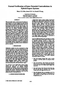
each pair of multipliers are equivalent. Table 7.1 shows the results for the veri cation of large n-bit multipliers built this may. We are able to verify pairs of multipliers up to 1024-bit to be equivalent. The original 16-bit multipliers are veri ed to be equivalent by pulling two variables (256gat and 290gat) up to the root. Each of the pairs of larger multipliers is veri ed by pulling the same two variables up to the root. No other knowledge of internal vertices is required. It is also possible to build and verify the multipliers by using multiple instances of c6288-c6288nr instead of using substitution, but it is more complicated. Pulling the two variables 256gat and 290gat up to the root works for one of the instances of c6288-c6288nr but not for all of the other ones. This is because the inputs to the dierent instances are not identical. The right two variables to pull up to the root for one of the 16-bit multipliers would be the wrong two variables for another of the multipliers. We get exponential growth. It is possible to lift the right variables up to the top of each of the instances. It requires knowledge of internal vertices in the BED. One 1024-bit multiplier contains 4096 instances of a 16-bit multiplier. Verifying the two 1024-bit multipliers to be equivalent would require pulling the correct two variables up in 4096 sub-BEDs. The example shows that using substitution is an advantage. 7.4.2 P-Cut

We test our p-cut method experimentally on three fault trees: cea9601, and wes9701. They are from CEA (French Military), Dassault Aviation (French aviation company), and Westinghouse (American nuclear das9601,

158

CHAPTER 7. EXTENDING BEDS z

+ x0

:=

x0 :=

x0 :=

x0

:=

y0 :=

y0 := 

y1

x1

x0

y2

y0

x2

: A 2n-bit multiplier created from one n-bit multiplier using substitution. x and y are the formal parameters for the multiplication cell which are replaced with the actual parameters x , x , y , and y .

Figure 7.8 0

0

1

n

32 64 128 256 512 1024

2

1

2

Ops Subst N CPU sec 6 505 8 192 26 665 1.6 9 827 40 960 75 070 3.1 16 447 172 032 270 275 8.6 29 783 696 320 1:05
10 29.5 56 401 2 793 472 4:19
10 119 109 643 11 192 080 14:3
10 408 total

6 6

6

: Verifying equivalence between two n-bit integer multipliers; one based on c6288 and one based on c6288nr from the ISCAS'85 benchmarks. Column Ops shows the number of operator vertices in the BED and column Subst shows the number of substitutions. Ntotal is the total number of vertices used in the veri cation. CPU is the veri cation time measured in seconds on a Sun UltraSPARC 1. Table 7.1

7.5. RELATED WORK

159

industry), respectively. All our experiments are run on a 500 MHz Digital Alpha. Table 7.2 shows the number of p-cuts of order 1, 2, 3 and 4 for the three fault trees as well as the runtimes in seconds to nd a BDD representation for the p-cuts using Up One. For these calculations, the size of the BED data structure never exceeded 20 MB of memory. No. of p-cuts Runtime [sec] Name 1 2 3 4 1 2 3 4 cea9601 0 0 1144 2024 2 27 122 683 das9601 0 47 80 446 1 2 11 75 wes9701 2 211 1079 54436 6 26 151 2000 : Number of p-cuts of order 1, 2, 3 and 4, and running times in seconds to compute them using the Up One transformation. Table 7.2

These results should be compared with the standard method (the Up All algorithm), which is unable to calculate the p-cuts for cea9601 and wes9701. The former could not be build using 300 MB while the latter could not be build in 48 hours. For das9601 it succeeds in building the BDD for the fault tree in about 2 hours. The variable orderings used in the experiments are the ones given in the anonymous data les. The standard method depends on the variable ordering, and using improved heuristics to determine a good initial variable ordering will de nitely improve the performance. However, the Up One method will also bene t from the use of an improved variable ordering heuristic. 7.5 Related Work Extending binary decision diagrams with operators has been done by other researchers. Section 2.4 mentions some of the new data structures. The most common operators are the Boolean connectives. Jeong et. al. use existential and universal quanti ers in their XBDDs [JPHS91]. Hett, Drechsler, and Becker add existential quanti ers to obtain a new method for BDD construction [HDB96, HDB97]. Most BDD implementations have algorithms for doing substitution and quanti cation. In this chapter we have added the same functionality to BEDs using new operators. One way of thinking of the operators is as a lazy evaluation: The operators are placed in the data structure but they are rst expanded or evaluated when it is needed.

160

CHAPTER 7. EXTENDING BEDS

The idea of giving the operators vectors as arguments is also known from standard BDDs. Most BDD implementations have quanti cation and substitution algorithms which allow substitution and quanti cation of vectors. The ESUB operator combines two dierent operations in the computation of [ EX ] : the existential quanti cation and the substitution. In BDD-based model checking, existential quanti cation and Apply are often combined. Combinations of this kind are very eective compared to performing the operations one by one. We refer to the papers [DR97] and [DR98] for a detailed description of p-cuts. The papers are also a good starting point for readers interested in Boolean reliability models and fault trees. 7.6 Conclusion In this chapter we have explained how to extend the Boolean Expression Diagram data structure with new types of vertices. We have given examples of existential and universal quanti cation vertices and of substitution vertices. Furthermore, we have presented an operator vertex, ESUB, combining existential quanti cation and substitution. We have shown what properties an operator must have in order to be implemented as a vertex type in the BEDs. The properties are not very strict: The operator must have a terminal case and it must distribute in some form over if-then-else. Furthermore, only a limited number of attributes are available per vertex. An operator with these properties can be implemented in the BEDs by minor modi cations to the Mk, Up One and Up All algorithms. As a more detailed example of a new type of vertex in the BEDs, we have chosen the PC operator. Based on this operator we proposed a new method to compute minimal truncated p-cuts. It makes it possible to compute minimal truncated p-cuts directly from the BED without ever constructing the BDD representation of the fault tree (that is often of gigabyte size). The experimental results show that our method has an advantage over the BDD methods.

Chapter 8

Conclusion In this thesis we have examined the use of the Boolean Expression Diagram data structure in the area of formal veri cation. We have selected a number of dierent problems domains for investigation. The rst problem domain was veri cation of combinational circuits. We considered both circuits described in a at way and circuits described in a hierarchical way. From a at description of two combinational circuits we obtained a Boolean formula which expressed the equivalence of the circuits. Using BEDs we decided whether the formula is a tautology (the two circuits are equivalent) or not a tautology (the two circuits are not equivalent). We examined the following methods for proving or disproving tautology: Up All : Similar to a standard BDD approach. The BED is converted to a BDD from the bottom up. The rewriting rules cannot be used during Up All. Up One : Construction of a BDD by top down conversion of a BED. The rewriting rules are important for the performance of Up One. St almarck : Reasoning-based method. As opposed to the other two methods, Stalmarck's method does not convert or change the formula it works on. In terms of speed, Stalmarck's method does not work well on circuits. However, it uses little memory. We have experimented with variable ordering heuristics. Both the Fanin and the Depth Fanout heuristics give good results. Based on our research and experiments, we see the following uses for BEDs in combinational circuit veri cation: 161

162

CHAPTER 8. CONCLUSION  Use BEDs as BDDs with Up All. The rewriting rules form a prepro-

cessing step which helps speed up the veri cation by reducing the size of the initial BED. Especially the combination of Up All, rewriting rules and the Fanin heuristic gives good results. Since the rewriting rules are used only as a preprocessing step, all BDD speci c techniques can be used in the construction of the BDD.  Use Up One to convert BEDs to BDDs. This method works best if the two circuits being compared have a high degree of structural similarity. For example, the two 16-bit multipliers in the ISCAS'85 benchmark suite are easily veri ed using Up One. Circuits described in a hierarchical way may be converted to at circuits and then veri ed by the techniques above. However, we have focused on exploiting the structural information in the hierarchical circuit descriptions. The main idea is to reuse previously calculated results. Our method works best if the two circuits being compared have similar hierarchical structures. The advantage is that instead of working with representations of the functionality of the circuits, we work with representations of the relation between the circuits. We call such a relation between the circuits for a cut-relation. In some cases, the cut-relation has a simpler BED/BDD representation than the functionality of the circuits. In cases where the hierarchical structure of the circuits are quite similar, the method performs well. For example, we have successfully veri ed large adder and multiplier circuits using this technique. Unfortunately, if the circuits have dissimilar hierarchical structures, then the cut-relation may become complex and the performance of our method degrades. The second problem domain is symbolic model checking. We have presented a method for CTL model checking based on xed-point iterations. We use quanti cation by substitution for the quanti cation whenever possible. Quanti cation by substitution works well with BEDs. Quanti cation of all state variables can be done in just one traversal of the BED. However, we still need to quantify out the inputs. For this purpose we use scope reduction rules to press the quanti ers as far down as possible in the formulae. Then we perform the quanti cation using Up One. Symbolic model checking is typically done using the BDD data structure where equivalence and satis ability checking are constant time operations. Other people have tried using SAT-solvers. In our method we combine BDDs and SAT-solvers. Our model checking method works best on examples that can be modeled

8.1. FUTURE DIRECTIONS

163

with few or no input variables. In such examples we can fully exploit quanti cation by substitution, and we are able to achieve results superior to those obtained by standard BDD model checking tools. A feature of our method is that is it good at detecting errors. Systems with input variables is a problem as we are not able to use quanti cation by substitution to quantifying out the input variables. We propose lfp-CTL as a means of model checking such systems. The lfp-CTL logic is weaker than CTL. However, the nature of the lfp-CTL logic is such that we (often) do not need to quantify out the inputs. The third problem domain is fault tree analysis. We have chosen to focus on the computation of p-cuts. A p-cut is a representation of the most likely reasons for system failure. We have extended the BED data structure to facilitate p-cut computation. Using Up One, we are able to gradually transform a BED for a fault tree to a BDD for the p-cuts. Our p-cut algorithm utilizes the fact that not all the information in a fault tree is necessary to nd the p-cuts. The standard method is to construct the BDD for the fault tree and then compute the p-cuts. However, the BDDs are often huge and in many cases it is not possible to construct them. Our method avoids the BDD construction by only concentrating on the parts of the fault tree which contribute to the p-cuts. The algorithm works best for short p-cuts. Because of complexity reasons it is not well-suited for longer p-cuts. However, this may not be a serious limitation since short p-cuts are the ones of practical interest. We have proposed a method for solving the satis ability problem based on BEDs. The algorithm BedSat uses splitting on variables to divide the problem into smaller pieces. The splits are done using Up One, which allows us to take advantage of the rewriting rules during satis ability checking. We have compared a simple implementation of BedSat with state-of-theart SAT-solvers. On satis ability problems from model checking, BedSat performs well. We have discussed what is needed for extending the BED data structure. The p-cut computation method is an example of such an extension. We have introduced other extensions, e.g., for quanti cation and substitution. 8.1 Future Directions In this dissertation we have explored ways for doing formal veri cation using Boolean Expression Diagrams. However, we have by no means covered everything. There are still many paths to follow and directions to go. The

164

CHAPTER 8. CONCLUSION

following is a list of some of the topics we think it would bene cial to explore further:  Combining Up One and Up All. We have explored Up One and Up All independently. However, it is possible to combine them. We see two main ways to do this: { Use Up One rst on a number of variables. Then switch to Up All to nish the BED to BDD conversion. We have suggested Up One-minimizing in Section 3.2.3. This may be a starting point for further research. { Use Up, which works as a mix of Up One and Up All. Since the size of BDDs is quite sensitive to how far closely related variables are from each other in an ordering, it may be possible to keep the size down by pulling closely related variables up together.  Our proposed SAT-procedure BedSat does not utilize premature backtracking. As a result it sometimes gets stuck { especially when working on unsatis able problem instances. We expect that the addition of premature backtracking to BedSat will make it more robust. It would also be interesting to compare BedSat with the SAT-solvers proposed by Giunchiglia and Sebastiani in [Seb94, GS99]. Their methods also work on non-clausal formulae.  Characterizing the CNF formulae produced by BED to CNF conversion and tune the SAT-solvers for such formulae. This has been done by Shtrichman [Sht00] for Bounded Model Checking.  Detect when we are getting close to a xed-point. After each iteration in the xed-point calculation we need to determine whether we have reached the xed-point or we should continue with another iteration. At the moment we convert the BEDs to either CNF or BDDs. However, it might be worth using SAT-solvers (CNF conversion) in the beginning and then switch to BDD conversion near the xed-point. This would require some metric which tells us how close we are to the xed-point. One possible metric is the number of states in the set dierence between two successive xed-point approximations in the xed-point iteration. This metric usually follows a bell-shaped curve: starts out low, increases, peaks, decreases. Based on such a metric we could skip some of the termination checks in the xed-point algorithms.

Appendix A

The BED Tool NAME

bed | tool for manipulating Boolean formulae as Boolean Ex-

pression Diagrams.

SYNOPSIS bed [-h] [-b m ] [-c n ] [-f script- le ] [ lename ]

DESCRIPTION bed is a program which allows the user to

manipulate Boolean formulae represented as Boolean Expression Diagrams (BEDs). A BED is a generalization of a Binary Decision Diagram (BDD) which can represent any Boolean circuit in linear space and still maintain many of the desirable properties of BDDs. This BED package contains a number of algorithms for transforming a BED into a reduced ordered BDD. One (called Up All) closely mimics the BDD apply-operator. Another (called Up One) can exploit the structural information of a Boolean circuit. AVAILABILITY bed can be obtained from the World Wide http://www.it-c.dk/research/bed/

Web at

OPTIONS

Options may appear in any order as long as they appear before the lename. 165

166

APPENDIX A. THE BED TOOL -h -b -c -f

Print a short help message. Reserve m megabytes of memory for the BED data structure. Reserve n megabytes of memory for a cache. Execute the semicolon-separated commands in the script le.

lename

Formula description, see le format below.

COMMANDS

The bed tool is used to manipulate Boolean formulae represented by the BED data structure. One typical use of it is to transform a BED into a (reduced and ordered) Binary Decision Diagram (BDD). There are dierent ways to do this: by using upall which mimics the standard BDD apply -call, by using upone to lift the variables up to the outputs one at a time, or by using upsome which lefts a set of variables to the outputs. Another usage is to determine satis ability of a function represented by a BED. This can be done with the bedsat command. A number of other commands are available to obtain information about the BED data structure. All available commands a listed below. The syntax of the arguments is described after each command. upall output-list

Lifts all the variables up over the operators thereby eliminating the operators and transforming the BED into a BDD. The resulting BDD is both reduced and ordered. The ordering used is the order in which the user has entered the variables in the circuit description le.

upone input-list output-list

Takes each variable at a time (starting from the rst one) from the input-list and lifts it up in each of the BEDs rooted by the nodes in the output-list. A variable is either lifted up until it reaches the top or until it reaches a node containing a variable previously lifted by the same upone command.

167 upsome input-list output-list

Lifts the variables in input-list up in each of the BEDs rooted by the nodes in the output-list.

anysat node

Returns a satisfying assignment for Boolean function represented by node. An assignment is a list of inputs which are true. All other inputs are false. The command only works if the BED is transformed into a BDD rst.

anynonsat node

Returns a non-satisfying assignment for Boolean function represented by node. This only works if the BED is transformed into a BDD rst.

satcount node

Returns the number of satisfying assignments for Boolean function represented by node. This only works if the BED is transformed into a BDD rst.

eval node assignment-list

Evaluates the Boolean function of a node given the list of input assignments assignment-list. assignment-list is a list of inputs enclosed in '[' and ']'. Inputs in the list are set to be true. All other inputs are false.

bedsat output-list

Determines whether each node represents a satis able function (result is 1), or it is unsatis able (result is 0). The variable sattime determines the maximum CPU time used per node.

addinput input-list

let

Adds one or more new inputs to the BED. This is useful when one wants to change the BED interactively. ID = expr Creates a new output de ned by the Boolean expression expr. This is useful when one wants to change the BED interactively. expr is a Boolean expression with the following syntax

168

APPENDIX A. THE BED TOOL expr

binop

! ID j (expr) j expr binop expr j expr < var > expr j not expr j exists ID . expr j forall ID . expr j expr [ ID := expr ] ! and j or j biimp j nand j nor j xor j imp j limp j nimp j nlimp

The operators bind as you would expect. imp is the implication operator, limp is left implication, nimp is negated implication, and nlimp is negated left implication. The expression expr < var > expr is the if-then-else operator where expr denotes the low-child and expr denotes the high-child. 1

2

1

2

unlet output gc

Removes the output from the BED. Garbage collection of unreachable nodes. This is also done automatically whenever bed is running out of BED nodes.

set option value

Sets the option to value. There are the following options: support

is either left or right. This option controls whether the support command make a left rst (low- rst) or right- rst (high- rst) traversal of the BED. Default is left.

value

reductions

is either on or off. This option controls whether to use the rewriting rules for the BEDs. Default is on. value

169 dot zero

is either on or off. This option controls whether edges going to 0 are printed with the dot command. Default is on. value

dot numbers

is either on or off. This option controls whether vertex identi ers (numbers) are printed with the dot command. Default is on. value

dot ranksep, dot nodesep, dot margin, dot fontsize, dot ratio

Parameters passed to the DOT program. See the manual for DOT for more information.

sort roots

is either on or off. This option controls whether the outputs (roots) are presented alphabetically to the user. Default is on. value

sattime

The maximum CPU time in seconds for each root with bedsat command. Zero indicates no limit. Default is 0 seconds.

displaytime

The CPU time of each command is printed whenever the command takes longer than value CPU seconds. Default is 10 seconds.

bedsize

is the size in megabytes for the internal representation of the BED data structure. Default is 3.81 corresponding to 200000 vertices. value

cachesize

is the size in megabytes for the internal cache. Default is 0.53 corresponding to 20011 entries. node-list [ > lename ] Outputs the BEDs rooted at nodes in node-list to the le lename in the DOT format. DOT is a graphdrawing program from AT&T which can be obtained from the web at value

dot

http://www.research.att.com/sw/tools/graphviz/

170

APPENDIX A. THE BED TOOL read lename

Reads a le containing a description of Boolean formulae in the format described below. Any previously read circuit is discarded. write [ lename ] Writes the BED to the le lename or to TMP.bed if no lename is speci ed. source lename

Reads and executes a script of commands. The commands must be separated by semicolons.

dump node - node

Prints all nodes between the two node s.

dumpnode node

Prints node and all nodes reachable from it.

inputs

Prints a list of all the inputs in the BED.

outputs

Prints a list of all the outputs in the BED.

foreach root do "command "

stat

Iterates through all roots in the BED. For each root, the command is executed with root replaced by the current root. Multiple commands can be separated by semicolons. [ bed j hash j outputs ] Prints statistical information about either the BED data structure, the hashing or the outputs. Default is bed.

support node

Returns the support of the Boolean function represented by node.

cd, pwd, ls exit

j

The standard UNIX commands. quit

In interactive mode these commands exit the program. In script mode the script is terminated and the program goes into interactive mode.

171 halt help

Quits the program both in interactive mode and in script mode. [command ] An online help function. Returns a short help for the command or, if no argument is speci ed, an overview of the available commands.

The command arguments: node

is a name of an output node or a number of an internal node.

node-list

is either a single node, a list of node s enclosed in '[' and ']' and separated by spaces, or * denoting a list of all outputs.

output-list

is either a single output name, a list of output names enclosed in '[' and ']' and separated by spaces, or * denoting a list of all outputs. is the name of an input node (a variable name).

input input-list

is either one input, a list of input s enclosed in '[' and ']' and separated by spaces, or a command returning a list of inputs. The commands available are either * denoting a list of all inputs (variables), support( node ) which returns the support of node, fanin( node ) which returns the Fanin ordering of inputs of node, and nally fanout( node ) which returns the Depth Fanout ordering of inputs of node.

BED FILE FORMAT

The bed tool supports a simple le format for storing BEDs. The format is meant to be computer-friendly, not easy to use for humans. A le in this format consists of three parts: inputs, assignments, and outputs. The input and output parts specify the

172

APPENDIX A. THE BED TOOL

inputs and outputs of the formulae. The assignments specify vertices in the BED. The syntax for the le format is: BED le inputs input-list input assignments assign-list assign var-assign op-assign misc-assign op misc-op outputs output-list

! ! ! ! ! ! ! ! ! ! !

inputs assignments outputs inputs input-list input input-list j input

ID

assign assign-list

assign assign-list j assign var-assign j op-assign j misc-assign

NO ID ite NO NO NO - op NO NO NO ID misc-op NO NO

not j and j biimp j nand j nor j or j xor imp j limp jnimp j nlimp j ESUB := j ? j ! outputs output-list

j

! ! ! ID NO output-list j ID NO

An ID is a series of one or more letters, numbers, and underscores, or any string in single quotes. A NO is a non-negative integer. Each assign de nes a BED vertex. The rst NO is a unique identi er for the vertex. A vertex must be de ned earlier in the le than a vertex which refers to it. The terminal vertices 0 and 1 are implicitly de ned and have unique identi ers 0 and 1, respectively. var-assign represents a variable vertex. The rst NO is a unique vertex identi er. The ID is the variable name. The last two NO's are the identi ers of the low and high children. op-assign represents an operator vertex. The rst NO is a

173 unique vertex identi er. The last two NO's are the identi ers of the low and high children. misc-assign represents a vertex in the extended version of BEDs described in Chapter 7. The rst NO is a unique vertex identi er. The ID is a variable eld. The two last NO's are the identi ers of the low and high children. The operators imp, limp, nimp, nlimp, and biimp are implication, left implication, negated implication, negated left implication, and biimplication. The operators :=, ?, ! and ESUB correspond to substitution, existential quanti cation, universal quanti cation and ESUB. The rest of the operators have standard names. The negation operator not takes two identical arguments. The substitution assignment denotes a Boolean function in which an input is replaced with another Boolean function. The existential (universal) quanti cation assignment denotes a Boolean function in which an input is existentially (universally) quanti ed. In this case the input is no longer free and thus not a real input anymore. However, it should still be listed in the input part. The outputs are speci ed as an ID and a NO. The ID is the name of the output. The NO is the unique identi er for a vertex in the BED. A full-adder can be speci ed like this inputs a b ci assign 2 a 3 b 4 ci 5 6 7 8 9 -

ite ite ite xor xor and and and

0 0 0 2 5 2 3 2

1 1 1 3 4 3 4 4

174

APPENDIX A. THE BED TOOL 10 11 outputs sum carry

or or

7 9

8 10

6 11

EXAMPLE 1

Consider verifying that two dierent implementations of a fulladder are logically identical. Let the full-adders be described by the following script: addinput a b ci; let s1 = (a and b and ci) or ((((a or b) and ci) nor (a and b)) and (a or b or ci)); let c1 = not (((a or b) and ci) nor (a and b)); let s2 = a xor b xor ci; let c2 = (a and ci) or ((a and b) or (b and ci));

The outputs of the two full-adders are combined using biimp operators: let sum_check = s1 biimp s2; let co_check = c1 biimp c2;

The outputs sum check and co check can be veri ed to be tautologies with the following commands upall sum check upall co check

or upone support(sum check) sum check upone support(co check) co check

175 All commands return 1 indicating a tautology. We now introduce an error in one of the full-adders by changing the line let s1 = (a and b and ci) or ((((a or b) and ci) nor (a and b)) and (a or b or ci));

to let s1 = (a and b and ci) or ((((a nor b) and ci) nor (a and b)) and (a or b or ci));

and run the script again. The upone and upall commands now return a value dierent from 1. The two circuits no longer implement the same Boolean function. The command anynonsat sum check

returns a falsifying assignment for sum check, for example [ ci ] which corresponds to the assignments a = 0, b = 0, ci = 1. Use eval on each of the s's to observe the dierent value for this assignment: eval s1 [ ci ] eval s2 [ ci ]

The rst command results in a 0, the second in a 1. EXAMPLE 2

Consider verifying that two multi-output combinational circuits are equivalent. Assume that the two circuits are described in the le circuits.bed in the BED le format. Each output in circuits.bed is a biimplication of two corresponding outputs from the original circuits. In other words, our veri cation task is to prove all outputs of circuits.bed to be tautologies. Write a script- le, script.com, containing the following commands:

176

APPENDIX A. THE BED TOOL foreach root do "order fanin(root); upall root"; stat outputs; halt;

Now run the bed tool with the following options: bed -f script.com circuits.bed bed reads circuits.bed and executes in turn each command in script.com. The rst command iterates through all outputs in circuits.bed. For each output it rst sets the variable or-

dering according to the Fanin heuristic. Then it calls Up All to convert the BED for the output to a BDD. After converting all output BEDs to BDDs, the script executes the command stat outputs which gives the number of tautologies among the outputs. In this way we can see whether the veri cation succeeded (all outputs are tautologies) or failed (some outputs were not tautologies). The command halt exits the bed tool. Change the foreach command in script.com to one of the following commands: foreach root do "order fanout(root); upall root"; foreach root do "order fanin(root); upone * root"; foreach root do "order fanout(root); upone * root";

The rst command will use the Depth Fanout heuristic and Up All. The remaining two commands will use Up One with the Fanin and Depth Fanout heuristics, respectively. The script script.com was used in the experiments presented in Tables 3.5 and 3.6.

Bibliography [ABE00]

P. A. Abdulla, P. Bjesse, and N. Een. Symbolic reachability analysis based on SAT solvers. In Tools and Algorithms for the Construction and Analysis of Systems (TACAS), 2000. 5.1, 5.3.1, 20, 5.6, 5.6 [AGD91] P. Ashar, A. Ghosh, and S. Devadas. Boolean satis ability and equivalence checking using general binary decision diagrams. In Proc. International Conf. Computer Design (ICCD), pages 259{264. IEEE Computer Society Press, 1991. 7 [AH] H. R. Andersen and H. Hulgaard. Boolean expression diagrams. Information and Computation. (To appear). 2, 2.2, 2.3, 2, 7 [AH97] H. R. Andersen and H. Hulgaard. Boolean expression diagrams. In IEEE Symposium on Logic in Computer Science (LICS), July 1997. 2, 2.2, 2.3, 6, 7 [Ake78] S. B. Akers. Binary decision diagrams. IEEE Transactions on Computers, 27(6):509{516, June 1978. 2.4 [BBS91] R. E. Bryant, D. L. Beatty, and C.-J. H. Seger. Formal hardware veri cation by symbolic ternary trajectory evaluation. In Proc. ACM/IEEE Design Automation Conference (DAC), pages 397{402, June 1991. 5.6 [BC95] R. E. Bryant and Y.-A. Chen. Veri cation of arithmetic functions with binary moment diagrams. In Proc. ACM/IEEE Design Automation Conference (DAC), pages 535{541, 1995. 2.4, 7, 7, 3.6 [BCC 99] A. Biere, A. Cimatti, E. M. Clarke, M. Fujita, and Y. Zhu. Symbolic model checking using SAT procedures instead of +

177

178

BIBLIOGRAPHY

BDDs. In Proc. ACM/IEEE Design Automation Conference (DAC), 1999. 3.2.3, 5.1, 5.3.2, 5.5, 5.6 [BCCZ99] A. Biere, A. Cimatti, E. M. Clarke, and Y. Zhu. Symbolic model checking without BDDs. In Tools and Algorithms for the Construction and Analysis of Systems (TACAS), volume 1579 of Lecture Notes in Computer Science. Springer-Verlag, 1999. 3.2.3, 5.1, 5.5, 5.6 [BCL 94] J. R. Burch, E. M. Clarke, D. E. Long, K. L. MacMillan, and D.L. Dill. Symbolic model checking for sequential circuit veri cation. IEEE Transactions on Computer-Aided Design of Integrated Circuits and Systems, 13(4):401{424, April 1994. 5.3.1 [BCM 92] J. R. Burch, E. M. Clarke, K. L. McMillan, D. L. Dill, and L. J. Hwang. Symbolic model checking: 10 states and beyond. Information and Computation, 98(2):142{170, June 1992. 5.1, 5.6 [BCRZ99] A. Biere, E. Clarke, R. Raimi, and Y. Zhu. Verifying safety properties of a PowerPC microprocessor using symbolic model checking without BDDs. In Computer Aided Veri cation (CAV), volume 1633 of Lecture Notes in Computer Science. Springer-Verlag, 1999. 3.2.3, 5.1, 5.5, 5.6 [BD97] B. Becker and R. Drechsler. Decision diagrams in synthesis { algorithms, applications and extensions. In VLSI Design Conference, pages 46{50, Hyderabad, January 1997. 2.4 [BF85] F. Brglez and H. Fujiware. A neutral netlist of 10 combinational benchmarks circuits and a target translator in Fortran. In Special Session International Symposium on Circuits and Systems (ISCAS), 1985. 3.2.4, 3.5.1, 22 [BFG 93] R. I. Bahar, E. A. Frohm, C. M. Gaona, G. D. Hactel, E. Macii, A. Pardo, and F. Somenzi. Algebraic decision diagrams and their applications. In Proc. International Conf. ComputerAided Design (ICCAD), pages 188{191, 1993. 7, 3.6 [Bje99] P. Bjesse. Symbolic model checking with sets of states represented as formulas. Technical Report CS-1999-102, Chalmers University of Technology, Sweden, June 1999. 3.2.3 +

+

20

+

BIBLIOGRAPHY

[Bra93]

179

D. Brand. Veri cation of large synthesized designs. In Proc. International Conf. Computer-Aided Design (ICCAD), pages 534{537, 1993. 10, 3.7, 3.6 [BRB90] K. Brace, R. Rudell, and R. Bryant. EÆcient implementation of a BDD package. In Proceedings of the 27th ACM/IEEE Design Automation Conference. IEEE 0738, 1990. 2.1 [BRRM91] K. M. Butler, D. E. Ross, R.Kapur, and M. R. Mercer. Heuristics to compute variable orderings for eÆcient manipulation of ordered binary decision diagrams. In Proc. ACM/IEEE Design Automation Conference (DAC), number 28, pages 417{ 420, 1991. 3.3 [Bry86] R. E. Bryant. Graph-based algorithms for boolean function manipulation. IEEE Transactions on Computers, 35(8):677{ 691, August 1986. 2, 2.2, 2.2, 2.2, 6, 2.4, 7, 3.5.1, 5.1, 7.4.1 [Bry92] R. E. Bryant. Symbolic boolean manipulation with ordered binary-decision diagrams. ACM Computing Surveys, 24(3):293{318, September 1992. 2, 2.2, 2.2, 6, 7 [Bry95] R. E. Bryant. Binary decision diagrams and beyond: Enabling technologies for formal veri cation. In Proc. International Conf. Computer-Aided Design (ICCAD), pages 236{ 243, November 1995. 2.4 [CBM89] O. Coudert, C. Berthet, and J.C. Madre. Veri cation of synchronous sequential machines using symbolic execution. In Proceedings of the International Workshop on Automatic Veri cation Methods for Finite State Systems, volume 407 of Lecture Notes in Computer Science, pages 365{373, Grenoble, France, June 1989. Springer-Verlag. 3.2.3, 5.3.1 [CCGR99] A. Cimatti, E.M. Clarke, F. Giunchiglia, and M. Roveri. NuSMV: a new Symbolic Model Veri er. In N. Halbwachs and D. Peled, editors, Proceedings Eleventh Conference on Computer-Aided Veri cation (CAV'99), volume 1633 of Lecture Notes in Computer Science, pages 495{499, Trento, Italy, July 1999. Springer-Verlag. 5.4 [CES86] E. M. Clarke, E. A. Emerson, and A. P. Sistla. Automatic veri cation of nite-state concurrent systems using temporal logic

180

BIBLIOGRAPHY

[CFZ95]

speci cations. ACM Transactions on Programming Languages and Systems, 8(2):244{263, April 1986. 5.2.1, 5.6

E. M. Clarke, M. Fujita, and X. Zhao. Hybrid decision diagrams overcoming the limitations of MTBDDs and BMDs. In Proc. International Conf. Computer-Aided Design (ICCAD), pages 159{163, Los Alamitos, Ca., USA, November 1995. IEEE Computer Society Press. 7 [CGP99] E. M. Clarke, O. Grumberg, and D. Peled. Model Checking. The MIT Press, Cambridge, MA, 1999. 16, 5.6 [CGS98] Marco Cadoli, Andrea Giovanardi, and Marco Schaerf. An algorithm to evaluate quanti ed Boolean formulae. In Proceedings of the 15th National Conference on Arti cial Intelligence (AAAI-98), pages 262{267, Menlo Park, July 1998. AAAI Press. 5.6 [CHP93] P.-Y. Chung, I. N. Hajj, and J. H. Patel. EÆcient variable ordering heuristics for shared ROBDD. In Proc. International Symposium on Circuits and Systems (ISCAS), pages 1690{ 1693, 1993. 3.3, 3.3.1 [CLR90] T. H. Cormen, C. E. Leiserson, and R. L. Rivest. Introduction to Algorithms. MIT Press, 1990. 2.2, 3.4.1 [CM90] E. Cerny and C. Mauras. Tautology checking using crosscontrollability and cross-observability relations. In Proc. International Conf. Computer-Aided Design (ICCAD), 1990. 3.6, 4.5 [CMZ 93] E. M. Clarke, K.L. McMillan, X. Zhao, M. Fujita, and J. Yang. Spectral transforms for large boolean functions with application to technology mapping. In Proc. ACM/IEEE Design Automation Conference (DAC), pages 54{60, 1993. 7, 3.6 [CW96] E. M. Clarke and J. M. Wing. Formal methods: State of the art and future directions. ACM Computing Surveys, 28(4):626{643, December 1996. 1.3 [DBR95] R. Drechsler, B. Becker, and S. Ruppertz. K*BMDs: a new data structure for veri cation. In IFI WG 10.5 Advanced Research Working Conference on Correct Hardware Design and Veri cation Methods, Frankfurt, Germany, October 1995. 7 +

BIBLIOGRAPHY

[DBR97a] [DBR97b]

[DLL62] [DP60] [DR97] [DR98]

[DST 94] +

[FFK88] [FMK91]

181

R. Drechsler, B. Becker, and S. Ruppertz. The K*BMD: A veri cation data structure. IEEE Design and Test of Computers, 14(2):51{59, 1997. 2.4, 7 R. Drechsler, B. Becker, and S. Ruppertz. Manipulation algorithms for K*BMDs. In Ed Brinksma, editor, Tools and Algorithms for the Construction and Analysis of Systems (TACAS), volume 1217 of Lecture Notes in Computer Science, pages 4{18. Springer-Verlag, 1997. 7 M. Davis, G. Longemann, and D. Loveland. A machine program for theorem-proving. Communications of the ACM, 5(7):394{397, July 1962. 5.6, 6.2, 6.5 M. Davis and H. Putnam. A computing procedure for quanti cation theory. Journal of the ACM, 7:201{215, 1960. 5.6, 6.2, 6.5 Y. Dutuit and A. Rauzy. Exact and truncated computations of prime implicants of coherent and noncoherent fault trees within aralia. Reliability Engineering and System Safety, 58(2):127{144, 1997. 7.3, 28, 7.3.2, 7.3.1, 7.5 Y. Dutuit and A. Rauzy. Polynomial approximations of boolean functions by means of positive binary decision diagrams. In Lydersen, Hansen, and Sandtorv, editors, Proceedings of European Safety and Reliability Association Conference, ESREL'98, pages 1467{1472. Balkerna, Rotterdam, 1998. ISBN 90 54 10 966 1. 7.3, 28, 7.3.1, 7.5 R. Drechsler, A. Sarabi, M. Theobald, B. Becker, and M.A. Perkowski. EÆcient representation and manipulation of switching functions based on ordered kronecker functional decision diagrams. In Proc. ACM/IEEE Design Automation Conference (DAC), pages 415{419, 1994. 7, 3.6 M. Fujita, H. Fujisawa, and N. Kawato. Evaluation and improvements of boolean comparison method based on binary decision diagrams. In Proc. International Conf. Computer-Aided Design (ICCAD), pages 2{5, November 1988. 3.3, 3.3.1 M. Fujita, Y. Matsunga, and T. Kakuda. On variable ordering of binary decision diagrams for the application of multi-level

182

[FOH93] [Fuj96] [GK00] [GKB97] [GM94] [Gra00] [GS99]

[Gup92] [Har96]

BIBLIOGRAPHY

synthesis. In Proc. European Conference on Design Automation (EDAC), pages 50{54, 1991. 5, 7 H. Fujii, G. Ootomo, and C. Hori. Interleaving based variable ordering methods for ordered binary decision diagrams. In Proc. International Conf. Computer-Aided Design (ICCAD), 1993. 3.3 M. Fujita. Veri cation of arithmetic circuits by comparing two similar circuits. In Computer Aided Veri cation (CAV), Lecture Notes in Computer Science, pages 159{168. SpringerVerlag, 1996. 1.3, 3.1 M. Ganai and A. Kuehlmann. On-the- y compression of logical circuits. In Proc. of International Workshop on Logic Synthesis, Dana Point, CA, June 2000. 3.6 E. I. Goldberg, Y. Kukimoto, and R. K. Brayton. Canonical TBDD's and their application to combinational veri cation. In Proc. International Workshop on Logic Synthesis, 1997. 3.6 J. Gergov and C. Meinel. EÆcient boolean manipulation with OBDD's can be extended to FBDD's. IEEE Transactions on Computers, 43(10):1197{1209, October 1994. 7, 3.6 H. Grauslund. Linear decision diagrams. Master's thesis, Department of Information Technology, Technical University of Denmark, Denmark, May 2000. Reference IT-E 843. 2.4, 7 E. Giunchiglia and R. Sebastiani. Applying the Davis-Putnam procedure to non-clausal formulas. In Proc. Italian National Conference on Arti cial Intelligence, volume 1792 of Lecture Notes in Computer Science, Bologna, Italy, September 1999. Springer-Verlag. 5.6, 6.5, 8.1 A. Gupta. Formal hardware veri cation methods: A survey. Formal Methods in System Design, 1(2/3):151{238, October 1992. 1.3 J. Harrison. Staalmarck's algorithm as a HOL derived rule. Lecture Notes in Computer Science, 1125:221{234, 1996. 3.5.3, 3.13

BIBLIOGRAPHY

[HC74] [HDB96] [HDB97] [HO82] [HWA97]

[HWA99] [JBA 97] +

[JMF95] [JPHS91] [KK97]

183

G. E. Hughes and M. J. Cresswell. An Introduction to Modal Logic. Methuen & Co. Ltd, London, 1974. 16 A. Hett, R. Drechsler, and B. Becker. MORE: Alternative implementation of BDD-pakages by multi-operand synthesis. In European Design Conference, 1996. 7, 7.5 A. Hett, R. Drechsler, and B. Becker. Fast and eÆcient construction of BDDs by reordering based synthesis. In IEEE European Design & Test Conference, 1997. 7, 7.5 C. M. Homann and M. J. O'Donnell. Pattern matching in trees. Journal of the ACM, 29(1):68{95, January 1982. 3.2.2 H. Hulgaard, P. F. Williams, and H. R. Andersen. Combinational logic-level veri cation using boolean expression diagrams. In 3rd International Workshop on Applications of the Reed-Muller Expansion in Circuit Design, September 1997. 1.5, 3 H. Hulgaard, P. F. Williams, and H. R. Andersen. Equivalence checking of combinational circuits using boolean expression diagrams. IEEE Transactions on Computer Aided Design, July 1999. 1.5, 3 J. Jain, J. Bitner, M. S. Abadir, J. A. Abraham, and D. S. Fussell. Indexed BDDs: Algorithmic advances in techniques to represent and verify boolean functions. IEEE Transactions on Computers, 46(11):1230{1245, November 1997. 7, 3.6 J. Jain, R. Mukherjee, and M. Fujita. Advanced veri cation techniques based on learning. In Proc. ACM/IEEE Design Automation Conference (DAC), pages 629{634, 1995. 3.6 S.-W. Jeong, B. Plessier, G. D. Hactel, and F. Somenzi. Extended BDD's: Trading o canonicity for structure in veri cation algorithms. In Proc. International Conf. Computer-Aided Design (ICCAD), pages 464{467, 1991. 7, 7, 3.3, 3.3.1, 7.5 A. Kuehlmann and F. Krohm. Equivalence checking using cuts and heaps. In Proc. ACM/IEEE Design Automation Conference (DAC), volume 34, pages 263{268, 1997. 3.6

184 [KP94]

[KPR96] [KSR92] [Kun93] [Lev99] [LPV94] [Mat96] [McM93] [Min93] [Min96]

BIBLIOGRAPHY

W. Kunz and D. K. Pradhan. Recursive learning: A new implication technique for eÆcient solutions to CAD problems { test, veri cation, and optimization. IEEE Transactions on Computer Aided Design, 13(9):1143{1158, September 1994. 3.5.1, 3.6 W. Kunz, D. K. Pradhan, and S. M. Reddy. A novel framework for logic veri cation in a synthesis environment. IEEE Transactions on Computer Aided Design, 15(1):20{32, January 1996. 10, 3.6 U. Kebschull, E. Schubert, and W. Rosenstiel. Multilevel logic synthesis based on functional decision diagrams. In Proc. European Conference on Design Automation (EDAC), pages 43{ 47, 1992. 7, 3.6 W. Kunz. HANNIBAL: An eÆcient tool for logic veri cation based on recursive learning. In Proc. International Conf. Computer-Aided Design (ICCAD), pages 538{543, 1993. 3.6 N. Leveson. Building safety into computer controlled systems. Talk at Carnegie Mellon University, November 1999. For more information, visit Dr. Leveson's website at http://sunnyday.mit.edu. 1.4 Y. T. Lai, M. Pedram, and S. B. K. Vrudhula. EVBDD-based algorithms for linear integer programming, spectral transformation and function decomposition. IEEE Transactions on Computer Aided Design, 13(8):959{975, August 1994. 7, 7 Y. Matsunaga. An eÆcient equivalence checker for combinational circuits. In Proc. ACM/IEEE Design Automation Conference (DAC), pages 629{634, 1996. 10, 3.6 K. L. McMillan. Symbolic Model Checking. Kluwer Academic Publishers, 1993. 5.1, 16, 5.2.2, 5.3 S. Minato. Zero-suppressed BDDs for set manipulation in combinatorial problems. In Proc. ACM/IEEE Design Automation Conference (DAC), pages 272{277, 1993. 7, 7.3 S. Minato. Binary Decision Diagrams and Applications for VLSI CAD. Kluwer Academic Publishers, 1996. 7, 3.3, 3.3.2

BIBLIOGRAPHY

[ML98]

185

J. Mller and J. Lichtenberg. Difference decision diagrams. Master's thesis, Department of Information Technology, Technical University of Denmark, Building 344, DK-2800 Lyngby, Denmark, August 1998. 2.4, 7 [MLAH99] J. Mller, J. Lichtenberg, H. R. Andersen, and H. Hulgaard. Dierence decision diagrams. In Proceedings 13th International Workshop on Computer Science Logic, volume 1683 of Lecture Notes in Computer Science, pages 111{125, Madrid, Spain, September 1999. 2.4, 7 [MSS99] J. P. Marques-Silva and K. A. Sakallah. GRASP: A search algorithm for propositional satis ability. IEEE Transactions on Computers, 48, 1999. 14, 5.3.2, 23 [MTJ 97] R. Mukherjee, K. Takayama, J. Jain, M. Fujita, J. A. Abraham, and D. S. Fussell. Flover: Filtering oriented combinational veri cation approach. In Proc. International Workshop on Logic Synthesis, May 1997. 10 [MWBSV88] S. Malik, A. R. Wang, R. K. Brayton, and A. SangiovanniVincentelli. Logic veri cation using binary decision diagrams in a logic synthesis environment. In Proc. International Conf. Computer-Aided Design (ICCAD), pages 6{9, 1988. 3.3, 3.3.1 [OYY93] H. Ochi, K. Yasuoka, and S. Yajima. Breadth- rst manipulation of very large binary-decision diagrams. In Proc. International Conf. Computer-Aided Design (ICCAD), pages 48{55, 1993. 7.4.1 [Pap94] C. H. Papadimitriou. Computational Complexity. AddisonWesley, New York, 1994. 28 [PPC96] D. K. Pradhan, D. Paul, and M. Chatterjee. VERILAT: Veri cation using logic augmentation and transformations. In Proc. International Conf. Computer-Aided Design (ICCAD), November 1996. 10, 3.6 [Ric98] M. Richards. A tautology checker loosely related to Stalmarck's algorithm. Talk at seminar given at Cambridge, March 1998. 3.6 +

186 [Rin99]

[Rud93] [S 92] +

[SDG95] [Seb94] [Sht00] [SLM92]

[Som98] [SS98]

BIBLIOGRAPHY

J. T. Rintanen. Improvements to the evaluation of quanti ed boolean formulae. In D. Thomas, editor, Proceedings of the 16th International Joint Conference on Arti cial Intelligence (IJCAI-99-Vol2), pages 1192{1197. Morgan Kaufmann Publishers, August 1999. 5.6 R. Rudell. Dynamic variable ordering for ordered binary decision diagrams. In Proc. International Conf. Computer-Aided Design (ICCAD), pages 42{47, 1993. 5 E. Sentovich et al. SIS: A system for sequential circuit synthesis. Technical Report Memorandum No. UCB/ERL M92/41, Electronics Research Laboratory, Dept. of EECS, University of California, Berkeley, 1992. 3.5.2 A. Shen, S. Devadas, and A. Ghosh. Probabilistic manipulation of boolean functions using free boolean diagrams. IEEE Transactions on Computer Aided Design, 14, 1995. 7 R. Sebastiani. Applying GSAT to non-clausal formulas. Journal of Arti cial Intelligence Research (JAIR), 1:309{314, January 1994. 5.6, 6.5, 8.1 O. Shtrichman. Tuning SAT checkers for bounded model checking. In Computer Aided Veri cation (CAV), volume 1855 of Lecture Notes in Computer Science, pages 480{494, Chicago, U.S.A., July 2000. Springer-Verlag. 8.1 B. Selman, H. J. Levesque, and D. Mitchell. A new method for solving hard satis ability problems. In P. Rosenbloom and P. Szolovits, editors, Proc. Tenth National Conference on Arti cial Intelligence, pages 440{446, Menlo Park, California, 1992. American Association for Arti cial Intelligence, AAAI Press. 5.6, 6.5 F. Somenzi. CUDD: CU Decision Diagram Package version 2.3.0. University of Colorado at Boulder, September 1998. http://vlsi.colorado.edu/fabio. 10 M. Sheeran and G. Stalmarck. A tutorial on Stalmarck's proof procedure for propositional logic. In G. Gopalakrishnan and P. J. Windley, editors, Proc. Formal Methods in ComputerAided Design, Second International Conference, FMCAD'98,

BIBLIOGRAPHY

[SW95]

187

Palo Alto/CA, USA, volume 1522 of Lecture Notes in Computer Science, pages 82{99, November 1998. 3.4, 3.6, 5.6

D. Sieling and I. Wegener. Graph driven BDDs { a new data structure for boolean functions. Theoretical Computer Science, 141(1-2):283{310, 1995. 7, 3.6 [US94] T. E. Uribe and M. E. Stickel. Ordered binary decision diagrams and the Davis-Putnam procedure. In J.P. Jouannaud, editor, 1st International Conference on Constraints in Computational Logics, volume 845 of Lecture Notes in Computer Science, September 1994. 3.6 [vE97] C.A.J. van Eijk. Formal Methods for the Veri cation of Digital Circuits. PhD thesis, Technische Universitet Eindhoven, 1997. 10, 3.6 [vE98] C.A.J. van Eijk. Sequential equivalence checking without state space traversal. In Proc. International Conf. on Design Automation and Test of Electronic-based Systems (DATE), 1998. 1.3, 3.1 [vEJ94] C.A.J. van Eijk and G. L. J. M. Janssen. Exploiting structural similarities in a BDD-based veri cation method. In Theorem Provers in Circuit Design, volume 901 of Lecture Notes in Computer Science, pages 110{125. Springer-Verlag, 1994. 3.6 [VPL96] S. B. K. Vrudhula, M. Pedram, and Y. T Lai. Edge Valued Binary Decision Diagrams. Kluwer Academic Publishers, 1996. 7, 7 [WAH01] P. F. Williams, H. R. Andersen, and H. Hulgaard. Satis ability checking using boolean expression diagrams. In T. Margaria and W. Yi, editors, Tools and Algorithms for the Construction and Analysis of Systems (TACAS), volume 2031 of Lecture Notes in Computer Science, 2001. 1.5, 6 [WBCG00] P. F. Williams, A. Biere, E. M. Clarke, and A. Gupta. Combining decision diagrams and SAT procedures for eÆcient symbolic model checking. In Computer Aided Veri cation (CAV), volume 1855 of Lecture Notes in Computer Science, pages 124{ 138, Chicago, U.S.A., July 2000. Springer-Verlag. 1.5, 5

188 [WHA99]

BIBLIOGRAPHY

P. F. Williams, H. Hulgaard, and H. R. Andersen. Equivalence checking of hierarchical combinational circuits. In IEEE International Conference on Electronics, Circuits and Systems (ICECS), September 1999. 1.5, 4 [Wil00] P. F. Williams. Formal Veri cation Based on Boolean Expression Diagrams. PhD thesis, Dept. of Information Technology, Technical University of Denmark, Lyngby, Denmark, August 2000. ISBN 87-89112-59-8. (document) [WNR00] P. F. Williams, M. Nikolskaa, and A. Rauzy. Bypassing BDD construction for reliability analysis. Information Processing Letters, 75(1-2):85{89, July 2000. 1.5, 7.3 [YCBO98] B. Yang, Y.-A. Chen, R. E. Bryant, and D. R. O'Hallaron. Space- and time-eÆcient BDD construction by working set control. In Asian-Paci c Design Automation Conference (ASPDAC), pages 423{432, February 1998. 3.5.1, 7.4.1 [Zha97] H. Zhang. SATO: An eÆcient propositional prover. In William McCune, editor, Proceedings of the 14th International Conference on Automated deduction, volume 1249 of Lecture Notes in Arti cial Intelligence, pages 272{275, Berlin, July 1997. Springer-Verlag. 15, 5.3.2, 23

Index apply, 23, 45 atomic propositions, 94 balancing, 41 BDD, 18, 28 BED, 13 algorithms, 20 free, 14 path, 16 reduced, 14 size, 16 support, 16 tool, 165 binary decision diagram, see BDD boolean expression diagram, see BED bounded model checking, 91 build, 84 cache, 23, 135 cell, 79 characteristic function, 6, 35, 80, 86, 99{101, 122 CNF, 73, 109, 132 combinational circuit, 33, 77 hierarchical, 77 computation, 95 computation tree logic, see CTL conjunctive normal form, see CNF connective, 4 container cell, 79 contradiction, 5 CTL, 95, 128 CTL*, 128 cut, 81 cut-relation, 81 Davis-Putnam, 132, 133

decision diagrams, 28 decomposition, 28 depth, 48 ESUB operator, 149 existential quanti cation, 142 ESUB operator, 149 vector, 145 fault tree, 151 nite state machine, see FSM FixIt, 114{116, 118 formal veri cation, 3 formal world, 3 FSM, 93, 95, 121 garbage collection, 18 Grasp, 92, 109, 127 hardness, 54 initial state, 102 input cut, 81 input relation, 81 instantiation, 80 interfaces, 8 ISCAS'85 benchmark, 43, 57 iterative squaring, 105 Kripke structure, 93, 121 lfp-CTL, 120 LGSynth'91 benchmark, 63 literal, 153 logic, 4 logic cell, 79 LTL, 128

189

190 minimal p-cut, see p-cut minimizing, 41 minterm, 153 model checking, 95, 101 monotonic, 97, 122 multiplier, 115, 156 negation normal form, 121 negative Davio, 28 NuSMV, 114, 115, 117, 118, 120 operator sets, 36 output cut, 81 output relation, 81 p-cut, 151, 153, 154, 157 path, 16, 81, 95 PC operator, 151, 157 positive Davio, 28 prime implicant, 153 product, 153 proof, 4 propagate, 84 property, 4 propositional logic, 4, 33, 50 pruning, 42 QBF, 5, 129 quanti cation by substitution, 103 quanti ed boolean formulae, see QBF quanti er, 5, 103 reactive system, 94 real world, 3 recursive learning, 62, 73 Reed-Muller, 28 reliability, 8 rewriting, 37 safety, 8 satis ability, 5, 108 satis ability problem, 5, 20 Sato, 92, 109, 114, 117, 127 scope reduction, 106 set inclusion, 104 set transformer, 97, 122

INDEX Shannon, 28 simpli cations, 36 SMV, 102, 110 speci cation, 4, 95 Stalmarck's method, 42, 50, 66 STE, 129 strong until, 96 substitution, 144, 156 vector, 147 symbolic trajectory evaluation, see STE system, 4 tautology, 5 tautology problem, 5, 20, 35, 131 temporal logic, 95, 128 transition, 94 transition function, 94, 102 transition relation, 94 universal quanti cation, 143 vector, 146 unsatis ability, 5 up, 25 up all, 23, 45 up one, 22, 45 variable ordering, 45 Depth Fanout, 49 Fanin, 48 weak until, 96