Signature: ...... addition, it can store the electrical energy in electrical vehicle system. [1, 76] and ...... switches, circuit breakers and relays of Smart Grid communicates ...... [87] "Powerline Related Intelligent Metering. Evolution (PRIME). [Online].
FORMAL VERIFICATION OF FAULT DETECTION AND SERVICE RESTORE SYSTEM IN SMART GRID USING PROBABILISTIC MODEL CHECKER
By Syed Atif Naseem
January 2018
Page | 1
FORMAL VERIFICATION OF FAULT DETECTION AND SERVICE RESTORE SYSTEM IN SMART GRID USING PROBABILISTIC MODEL CHECKER
A THESIS SUBMITTED TO THE GRADUATE SCHOOL OF NATURAL & APPLIED SCIENCES OF IZMIR UNIVERSITY OF ECONOMICS
BY
SYED ATIF NASEEM
JANUARY 2018
Page | 2
Page | 3
Dedication
To My Parents & Siblings
Page | 4
Certificate of Originality I would like to affirm that this thesis is the product of my individual efforts and no material is published before in any institute, journal by any other student or individual one. This thesis is my unique effort and never published in Izmir University of Economics for the requirement of master degree. I also affirm that the research material of the dissertation is my personal effort and the concept of this research has never been published in any journal or website.
Author Name: Syed Atif Naseem Signature:___________________
List of Publications from the Current Work: 1. Syed Atif Naseem, Riaz Uddin, Osman Hassan and Diaa E. Fawzy, "Probabilistic Formal Verification of Communication Network-based Fault Detection, Isolation and Service Restoration System in Smart Grid," Journal of Applied Logic (Accepted), 2017. (Hint: The paper is attached to the thesis).
Page | 5
Acknowledgment It’s my privileged to have Dr. Diaa Gadelmavla as my supervisor and mentor who guided me throughout the project and had given me an opportunity to do the research on this unique idea. I would also like to pay thanks to my parents for their support throughout the project and give me confidence to complete the thesis within the duration. I humbly pay thanks to Dr. Riaz Uddin from NEDUET for his guidance and Dr. Usman Hassan from NUST University.
Page | 6
Abstract Distribution Management System (DMS) starts with the expansion of Supervisory Control and Data Acquisition (SCADA) from the transmission grid behind the distribution grid. The Fault Detection, Isolation, and Service Restoration (FDIR) technique (DMS) form one of the most commonly used application today in Smart Grid. FDIR requires a higher level of optimization for closed-loop, parallel circuit, and radial configurations. FDIR is mainly employed to improve system’s performance after detecting the fault on a feeder section of the substation. Then, it trips off the faulty switch from the feeder and restores the service by directing the power to the faultless feeder sections. In this way, the restoration time of the distribution system reduces from a number of hours to a few seconds; significantly recovering the network by providing high quality of reliability and stability in the distribution system. Thus, the FDIR process requires some guarantee to work properly according to the conditions in real time. In this regard, the major contributions of this thesis are (i) to develop the Markov model of the FDIR behavior in distribution network of Smart Grid, (ii) formally verify the model in PRISM model checker tool in order to analyze the system’s (a) accuracy, (b) efficiency and (c) reliability by developing logical properties in PRISM tool. (iii) More-over the Markov models of the mechanisms of sending/receiving the data packet (IEEE 802.11 DCF) and G-3 power line communication are also developed and integrated with FDIR in PRISM model checker to investigate the overall system behavior. Another main purpose is to construct the probabilistic Markov model of FDIR along with the communication network to (iv) analyze the probabilistic frequency of fault occurrence in distribution network and (v) to predict the failure probability of the different components of distribution network in order to take a corrective action and maintenance. So that, the faulty component can be manually replaced Page | 7
in advance to avoid the complete failure of system. Moreover, we also (vi) analyze and predict the probability at which the load switches of distribution network function properly by making the faulty component detach itself upon the occurrence of fault. Finally, (vii) the prediction of the probability to recover the system through particular non-active switch is also analyzed along with the comparison between FDIR model with wireless communication network and FDIR model with ideal communication network such as Ethernet or fiber-optics medium. The simulation results show that increasing the restoration time period increases the probability by a factor of 0.03. We also expands the FDIR model by including 6 load switches, protection relay, circuit breaker and tested the FDIR behavior on Tianjin electric power corporation. The Markov model of expanding the network is thus interpreted on PRISM tool and verified the model through the temporal logic specification of PRISM model checker and predict the failure, isolation and restoration probabilities of component of Smart Grid. The comparison results are obtained and discussed when FDIR is connected with ideal communication medium as compared to FDIR connected with wireless communication network, which clearly shows that ideal communication network has less failure probabilities in Smart Grid compared to wireless communication medium.
Page | 8
Table of Contents 1
Introduction
1.1 Motivation……………………………………………………....14 1.2 Literature Review ………………………………………………16 1.3 Current Approach ……………………………………………..19 1.4 Thesis Contribution …………………………………………….21 1.5 Organization of Thesis …………………………………………22 2 Preliminaries 2.1 Model Checking………………………………………………. 24 2.2 Probabilistic Model Checking ………………………………….27 2.3 PRISM Model Checker ………………………………………...28 2.4 Smart Grid ……………………………………………………...29 2.5 Fault Localization, Isolation and Restore behavior for Smart Grid……………………………………………………………..31 2.6 Tianjin Electric Power Corporation…………………………….34 2.7 Communication Networks……………………………………..40 2.8 Justification of the model of FDIR…………………………….47 3 Proposed Methodology 3.1Modeling FDIR algorithm in PRISM...........................................48 3.2 Discrete Time Markov Model………………………………….50 3.3 Functional Verification using Simulation ...……………………68 3.4 Formal Function Verification . . . . . .…………………………..69 4 Simulation & Formal Function Verification Results 4.1 Simulation & Results of Case 1:FDIR with three Load Switches.72 4.2Simulation & Results of Case 2: FDIR with six Load Switches...84 4.3Simulation & Results of Case 3: FDIR with wireless communication medium…………………………………………….94 5 Conclusion……………………………………………………..102 Page | 9
6 Appendix A……………………………………………………104 7 Appendix B……………………………………………………113 8 Appendix C……………………………………………………128 9 Bibliography…………………………………………………...142
Page | 10
List of Table 1. A Comparison Between Previous Studies and Current Work
20
2. Markov Model
28
3. Summary of Results of Probability Estimation from PRISM
84
4. Summary of Results of Probability Estimation from PRISM
93
Page | 11
List of Figures Fig. 1 Model Checking
25
Fig. 2 Smart Grid
30
Fig. 3 State of IED
33
Fig. 4 Tianjin Electric Power Distribution Network
36
Fig. 5 Substation A of Tianjin Distribution Network
36
Fig. 6 Substation B of Tianjin Distribution Network Fig. 7 Substation C of Tianjin Distribution Network Fig. 8 Switching Station of Tianjin Distribution network
37 37 38
Fig. 9 Switches of Substation A of Tianjin Distribution
38
Fig. 10 Switches of Substation B of Tianjin Distribution Network 39 Fig. 11 Switches of Substation C of Tianjin Distribution Network 30 Fig. 12 Switches of Substation C of Tianjin Distribution Network 40 Fig.13 Tianjin Electric Power Network showing Wireless Communication Link 43 Fig.14 Tianjin Electric Power Network showing Power Line Communication Link 45 Fig. 15 Coupling Network
46
Fig. 16 Proposed Methodology
50
Fig. 17 Working of Probabilistic Models
51
Fig. 18 Fault Detection Model Fig. 19 Fault Isolation Model
54 55
Fig. 20 Supply Restoration Model
56
Fig. 21 Fault Localization Probabilistic Model (6 Load Switches) 58 Fig. 22 Fault Isolation Probabilistic Model (6 Load Switches) 60 Fig. 23 Supply Restoration Model 62 Fig. 24 Supply Restoration Model
63 Page | 12
Fig. 25 Communication Protocol at MAC layer of Communication system 67 Fig. 26 Receiving Station of the Communication System
68
Fig. 27 Simulator of PRISM Model Checker Fig. 28 Simulation Result of FDIR (Three Load Switches) Fig. 29 Result of the Dead Lock property
69 73 75
Fig. 30 Result of Detection of Fault Current
76
Fig. 31 Result of Fault Isolation Model Turned On Fig. 32 Result of No Two Process Run At Same Time
77 78
Fig. 33 Result of Restoration Model Not Take More Than 60 s
79
Fig. 34 Probability that Fault will Occur in Load Switch
80
Fig. 35 Probability of Fault Flag present at Switch 2
81
Fig. 36 Probability that Switch Trip-off at the Limited time
82
Fig. 37 Probability to Recover the Network
83
Fig. 38 Simulation Result (6 Load Switches)
85
Fig. 39 Result of Dead Lock Property
87
Fig. 40 Result of Detection of Fault Current
87
Fig. 41 Result of Fault Isolation Model Turn On Fig. 42 Result of No Two process Run at the Same Time Fig. 43 Probability that Fault will Occur in Load Switch
88 88 91
Fig. 44 Probability that Switch Trip-off at the Limited Time
92
Fig. 45 Probability to Recover the Network
92
Fig. 47 Fault Occurrence Probability of Switch # 1 Fig. 48 Fault Flag 2 Probability of Switch# 2
95 97
Fig. 49 Probability of Switch Tripping-off within the limited time 97 Fig. 50 Probability to Recover the System through Switch # 3 98 Fig. 51 Probability to Send the data by IED of CB 98 Page | 13
Fig. 52 Comparison of Probabilities for Failure of Components
99
Fig. 53 Components Tripping off Probabilities
100
Fig. 54 Load Switch Restoration Probabilities
101
Fig. 55 Tie Switch Restoration Probabilities at Different Time
101
Page | 14
Abbreviations FDIR FTU DAS CB DFA SDSI SDPI FASM ISOM RESM ACMP ACSP IED DTMC CTMC MDPs PTAs LTL CTL PCTL SCADA DMS
Fault Localization, Isolation & Supply Restoration Feeder Terminal Unit Distribution Automation System Circuit Breaker Distributed Feeder Automation Switch Data Service Instance Switch Data Proxy Instance FDIR Start Message Isolation Result Message Restoration Result Message Available capacity Message of Main Power Source Available Capacity Message of Standby Power Source Intelligent Electronic Device Discrete Time Markov Chain Continuous Time Markov Chain Markov Decision Process Probabilistic Timed Automata Linear Temporal Logic Computation Tree Logic Probabilistic Computation Tree Logic Supervisory Control And Data Acquisition System Distribution Management System
Page | 15
Chapter 1 Introduction 1.1
Motivation
With Smart Grid, confidence and expectations are high to deliver better services as compared to the conventional grid. Utility companies are expected to transform the existing grid which is unidirectional into bi-directional power grid aiming energy will be stored in electrical system and used where-ever it is necessary [1]. Formal analysis and verification of FDIR in Smart Grid is a unique and pioneer work as no one has ever performed it in probabilistic model checking environment. Safety-critical applications in Smart Grid such as demand response, home area network, distribution automation and energy storage etc., [2-10] need accurate modeling and analysis of such systems. These applications are of principle significance since a slight fault in design can outcome in severe consequence even at the cost of individual life and property. The ominous need for correct analysis and modeling have given rise to a variety of techniques [11-18] which were evolved over the time. Usually paper-and-pencil based approaches [11, 12] were found relatively perfect. However, as the systems grow in mass, the complexity increased as well, resulting in the scalability matter that made it complicated to guarantee the appropriateness of large mathematical proofs due to human error [19, 20]. The arrival of computers led to a new period of modeling and investigation, which lead to a large figure of techniques generally categorized as simulation based techniques [13] and computer-aided tool [14, 15]. The core of imitation depending on systems is to construct the discrete representation [21] to the real world structure and estimate the productivity of structure from a deposit of specified input samples. On the other hand, Computer Algebra Systems (CAS) [16, 17] ensured better results as compared to numerical methods-based simulations such as the approach [18] developed and verified a Page | 16
mathematical model corresponding to the real world system [22] but this system lacked absolute correctness because the computed results are not always mathematically correct. In order to overcome these limitations, we proposed the usage of formal verification in the safety-critical domain (whose failure may result in loss or severe damage to human/equipment/property). There are some advantages of using formal methods [23, 24] as they bridge the fissure between the conventional strong mathematical paper-andpencil approach [12] and current CAD tool design [25]. A major subject to build an arithmetical representation related to the genuine structure is very important. Once the arithmetical representation of any system is constructed, then it formally verify with in a computer by using the formal verification tools in order to find the design errors in a system [26]. Basically formal verification of a system [23, 26] can be done in three different ways based on its reason, judgment, self-expression and clarity. Theorem proving, symbolic simulation and model checking are the three methods often used to verify the reactive system and stochastic process [27]. In model checking a mathematical model is then translated to in the language of model checker and the linear temporal logic (LTL), computation tree logic (CTL) or probabilistic computation tree logic (PCTL) property [28] is fed to in the model checker along the translated mathematical model which gives the true result, if the model satisfies the temporal logic property, otherwise false result with counter example will be given by the model checker. In addition, model checking can be used to verify the Markovian model by providing the probabilistic temporal logic specification via PRISM and predict the probability of faults occur in a system and also predict how to restore it within a limited time as given in [29, 30]. On the other hand, theorem proving [31] is a very common approach and extensively used in verifying the characteristics of real world system. The classification of a system which represent the model should be in the mathematical form of suitable reason and the properties of significance are verified through computer tool called ‘theorem prover’ [31] whereas symbolic simulations filled the fissure between the conventional simulation and formal verification. The key Page | 17
initiative is to apply symbols as a substitute of real standards in simulating environment and execute the system multiple times [27] in order to reduce the number of test cases and simulate the system with reliability and effectively. Up till now, probabilistic formal verification of FDIR has never been performed for the study and analysis of FDIR classification in distribution network of future/Smart Grid. However a number of approaches were used to implement FDIR in distribution system but no one performed the probabilistic verification as summarized in the Table 1 of Section 1.2. 1.2 Literature Review Up to our knowledge, probabilistic model checker has never been used for the analysis and verification of fault detection, isolation and service restoration system (FDIR) in Smart Grid. However, there are varieties of approaches to implement them into the distribution network such as [32-37]. The approach in [33] includes FDIR system to show the comparison between a centralized architecture and decentralized architecture. It further explains the fault detection, isolation and service restoration functions in Smart Grid. It also discusses the use of re-closer [38] versus load break switches [39] for FDIR switching. In [34], service restoration planning discusses the simultaneous restoration scheme (after outage) with the sequential restoring system that controls the array of restoration and executes the restoration of every blackout individually. In case of failure to discover the possible arrangement to repair entire blackout load then simultaneous restoration design is useful [35]. Some researches by means of decentralized structural design to accomplish the FDIR, depends on Multiple representative structure knowledge [36] and provides details on multiple representative structure to recover an energy scheme after an error occurred in the system. It has different kinds of agents and by means of JAVA agent development framework (JADE) as a multiple-representative structure to swap the order and verify the possible renovation approach. Furthermore, the work in Page | 18
[37] introduced a multi agent system (MAS) design to develop the consumer examine restoration for the error occurrence possibility of substation. It separately defines the process system for possible error occurrence in feeder, service restoration for main transformer fault and load shedding rules. The approach in [40] proposed a control structure of automation based on circulated intelligence along with a technique of integrating the IEC 61850 and IEC 61499 [40]. Furthermore, it discusses about the power system equipment, protection and automation through supervisory control and data acquisition system (SCADA). The multiagent approach in [41] proposes the decentralized restoration scheme for a substation of distribution network. It is composed of a numerous feeder agents and load agents while feeder agents perform as an administrator for result procedure. Another MAS in [42] introduces architecture and its design for restoration scheme and proposes three types of agents i.e., facilitator agent, bus agent and load agents. It also discusses the drawback of centralized control system i.e., supervisory control and data acquisition system (SCADA) over multi agent system (MAS) for the timely solution of the restoration purpose on a vast level. In [43] a substation restoration technique applying multiagent is projected for escalating the effectiveness and reduction moment of the restoration of power failure. The approach in [44] proposes the shortening of the restoration time from minutes to seconds by using MAS in order to increase its operational reliability. The scheme in [45] offered the multi-agent structure to establish a defective region and segregate the error by examining the limited ampere and interchanging it with the neighbor switches. To communicate the intelligent electronic device (IEDS) of different power components of Smart Grid with each other, different communication network such as Ethernet, Wifi, PLC etc., are used and in this regards, [46] discusses the coupling network of communication network with power network and analyzes the IEEE test cases (9, 14, 30, 118, 300 bus case) of different sizes network with the communication network. The main theme in this work is to find the probability of Page | 19
communication network failure on two different timing condition i.e., 3ms and 10ms. It also suggests that the probability of failure of Ethernet communication network is much lower as compared to wireless communication network. The work in [47] proposes the multi-hop wireless network with a frequency-reprocess configuration of cellular network and addresses the challenges to send and receive the huge information in future grid applications. It presents the system planning for analyzing the reporting of network and capability. The work in [48] describes the wireless Smart Grid communication system and explain the home area network in which the sensors are installed in the home appliances and form the wireless mesh network with the neighborhood area network and transmits the data through the wide area network (WAN) access point in order to receive the data at the control centre of the Smart Grid. The work also inspects the topologies of networking and wireless data packet simulation result is also shown. In [49], the important issues on Smart Grid technologies specifically related to the communication network technology and information technology network are discussed and provides the present situation regarding the ability of Smart Grid communication system. Study by [50] analyzes the reliability and resilience of Smart Grid communication network by using the IEEE 802.11 communication technology in both infrastructure single-hop and mesh multiple-hop topologies for upgraded meters in a system called building area network (BAN). Another study in [51] proposes the wireless mesh network for a smart distribution grid and then analyzed the security framework under this communication architecture. In addition to the wireless communication network to make a reliable communication link between the IEDS of different element of the substation of future grid, a vast number of studies is presented to show that communication of IEDS through power line communication is possible and suggests that it is a more reliable medium as compared to other communication technologies. In this regard, [52] proposes a narrow band power line communication (PLC) network for outdoor communication component from smart meters to data centers on low voltage or medium voltage power lines Page | 20
in the 3-500 kHz spectrum band. It also presented detailed information on the different types of interferences occurred over the power lines which degrade the quality of communication system of the Smart Grid. The work in [53] develops an iterative algorithm called water filling for PLC system in order to analyze the multichannel modulation techniques. It also describes the different kinds of noises available at the PLC channel; the power spectral density phenomenon is used to represent the intensity of channel noises. In [54], the general model of the broadband PLC network architecture is presented to connect the high voltage lines, substation and low voltage lines at the consumer end. It also proposes the algorithm called recursive to approximate the carrier frequency equalization, and its performance is evaluated through the maximum likelihood approach. Another work in [55] presents the overview on PLC system from two different standards i.e., IEEE and ITU (International Telecommunication Union), which presents the similarities and dissimilarities between these two standards. This paper also gives detailed information on physical layer specification and MAC protocol of PLC network of both standards respectively. Work in [56] suggested a solution to integrate two heterogeneous network architectures by combining PLC with the back bone of IPbased network. It also discussed the critical issues of energy management application by highlighting the reliability, availability, coverage distance, communication delay and security standard of communication network. Work in [57] presents a solution to integrate the active management system in the network infrastructure when number of distribution and generation setups are involved in the substation of Smart Grid. It also discussed the standard protocol and technology of different communication network in terms of data rate, bit error rate and installation cost of each wired and wireless medium. 1.3 Current Approach From the literature review, we can conclude that formal verification of FDIR has not been done before and to support our claim, we summarize previous studies in table 1. Page | 21
Fault Detection , Isolation & Restoration System (FDIR)
Techniques Compare centralized & decentralized architecture
Literature
Formal Verification
[33]
No
Restoration scheme
No [34]
Decentralized structure
No [35]
Different kinds of agents to restore power system MAS design for restoration
[36]
No
No [37]
Integration Of technique
No [40]
Restoration scheme
[41]
Restoration scheme
No
No [42]
Substation restoration technique
[43]
Shortening of restoration time
[44]
No
No
Page | 22
Monitoring the limited current
No [45]
Table. 1 A Comparison Between Previous Studies and Current Work 1.4
Thesis Contribution
Keeping the above issues in iterative- or simulation-based method in mind, and for achieving the absolute correctness and system reliability analysis in real world problem, this motivated us to use the formal methods [23, 24] in the safety critical domain (whose failure may result in loss or severe damage to human/equipment/property). The current method verified the model and takes out the errors after rigorous verification of the model through temporal logic specification. Up till now, probabilistic formal verification of FDIR along with communication network has never been performed for the study and verification of FDIR classification in distribution network of future/Smart Grid. However a number of approaches used to implement FDIR in distribution systems but no one performed the probabilistic verification as summarized in the table 1. On the other hand, the above mentioned FDIR approaches in Table 1, mainly discussed the restoration of fault in distribution network but they did not give any idea on switching and communication failures (possibly in terms of probabilities) of FDIR in distribution network with communication networks such as Ethernet, wifi. Some preventive actions may be designed for fast isolation and restoration of Smart Grid system. This mainly motivated us to analyze the switching failure of FDIR component along with the failure probability of communication network in order to determine the expected time required to recover a system after the switching fault or communication fault has occurred in FDIR of Smart Grid. Furthermore, the above approaches in table 1 also did not perform any formal verification on FDIR in their respective system which is Page | 23
important to verify the switching and communication logics among different components in a distribution network of Smart Grid. In order to implement our proposed formal verification notion, we performed the following task (i) a Markovian representation of FDIR for an established Tianjin Electric Power Corporation network [58] is integrated along with a mechanism of sending/receiving the data packets (IEEE 802.11 DCF) (considered as Smart Grid). (ii) This Markovian FDIR model is employed in PRISM [59] model checker tool to formally verify the system accuracy, availability, efficiency and reliability with wireless communication network. Furthermore, several more important studies (contributions) such as (iii) the comparison between FDIR model with wireless communication network and with ideal communication network such as Ethernet or fiber-optics is performed and (iv) the probability of (a) switching and communication failures of FDIR in any distribution network / Smart Grid (b) tripping-off the switch within the limited time period (c) to recover the system automatically within the least possible time after the occurrence of fault is also predicted and discussed in detail. 1.5
Organization of Thesis
The thesis is organized as follows: chapter 2 provides an outlines on model checking, probabilistic model checking, PRISM model checker, Smart Grid, fault detection, isolation and restoration system along with the brief introduction of Tianjin Electric Power corporation, communication networks and justification of FDIR model. The proposed methodology adopted for the verification of FDIR in Smart Grid and developed the Markov model of FDIR along with communication network and several properties are proposed to analyze the behavior of FDIR system in Smart Grid is discussed in details in chapter 3. Chapter 4 gives the simulation and formal verification results of different cases, when FDIR connected with three load switches, FDIR connected with six load switches and FDIR integrated with wireless/ power line communication network. Finally, chapter 5 concludes the thesis and point out the key contribution of the thesis. Page | 24
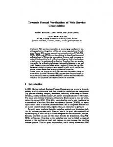
Chapter 2 Preliminaries Summary: This chapter presents the general overview and basic background information on model checking, formal verification method, probabilistic model checking and PRISM model checker. It also gives a brief overview of Smart Grid, fault detection and restoration system, Tianjin Electric Corporation network along with communication system which is formally verified in the thesis. 2.1 Model Checking Literature [28] defines the principles of model checking and stated that the model of the complex systems can be verified through temporal logic property within the computer system. It takes a lot of time in verifying the complex model instead of constructing the model. Model checking overcomes the limitation of simulation as it is not possible to check and verify all the scenarios and performance of the specified structure through physical testing and simulation. It is the drawback of simulation that it cannot verify all the possible higher number of cases as it is non exhaustive in nature and therefore failure cases may occur due to not simulated the all scenarios/possibilities. In model checking, we capture the behavior of real world system and transform it into finite state machine. A finite state machine is basically the Markovian model of the real world system in which each state proceed to another state of the model by satisfying the condition and probability of the current state. This Markovian model is then translated to in the language of model checker and fed to in the tool. The temporal logic property is basically a condition through which we are interested to satisfy the model. LTL, CTL, PCTL are the commonly used temporal logic property which we develop and fed in Page | 25
to the model checker to test the model exhaustively and give us a true result if the condition i.e temporal logic property satisfy the model or otherwise sends the counter example. The model checking phenomenon to test the model through temporal logic property is shown in fig. 1
Fig. 1 Model Checking (Source : [28] ) Some of the generally used model checking tool is SPIN model checker which is suitable to analyze the distributed system. For synchronized system i.e digital system software and hardware NUSMV is the tool to analyze such system. UPPAAL is the software used to study and investigate the real time system and HYTECH tool is used for hybrid system where PRISM is used to create and analyze the probabilistic type model.
Page | 26
2.1.1 Formal Verification Method In order to achieve the absolute correctness and system reliability analysis in real world problem, we use the formal methods [24, 25] in the safety critical domain which test the model and takes out the errors after rigorous verification of the model through temporal logic specification. Formal methods basically build an arithmetical representation related to the genuine classification and then formally verify the accuracy and precision of the mathematical model within a computer through temporal logic specification which in turn increases the probability of finding design errors. A mathematical model is then translated to in the language of model checker and LTL, CTL or PCTL property is fed to in the model checker along the translated mathematical model which gives the true result, if the model satisfies the specification otherwise false result with counter example given by the model checker. Basically formal verification of systems can be done in three different ways based on its reason, judgment, self-expression and clarity. Theorem proving, symbolic simulation and model checking are the three tools often used to verify the reactive system and stochastic process. 2.1.2 Theorem Proving Theorem proving is very common approach and extensively used in verifying the characteristics of real world systems. The classification of system which is necessary to realize should represent the model in the mathematical form of suitable reason and the properties of significance are verified through a computer tool called ‘theorem prover’. 2.1.3 Symbolic Simulation Symbolic simulation filled the fissure linking the conventional simulation and formal verification. The key initiative is to apply Page | 27
symbol as a substitute of real standards in a simulation environment and execute the system multiple times. 2.2 Probabilistic Model Checking A classification that exhibits random behavior, probabilistic model checker is used [60], [61] for the formal study and verification of such system and therefore can be represented as Markov chains [62]. However, depending upon its nature, application and usefulness, a system behavior which is probabilistic in nature is represented as discrete time Markov chain (DTMC) [29], continuous time Markov chain (CTMCs) [63], Markov decision process (MDPs) [64] and probabilistic timed automata (PTAs) [65], [62]. In DTMC the present state move to next state by fulfilling certain conditions with the applied probabilities, whereas in CTMC the present state transit to next state does not depend only the probabilities to make such transition but also include the delay before making the transition and move to the next state. These random delays usually are represented as exponential probability distribution [62]. MDPs and PTAs are with non-deterministic transitions whereas DTMCs and CTMC are fully probabilistic transitions. Table. 2 shows the difference among these Markov models. Once the probabilistic Markov model of the random behavior of system is finalized, the verification and analysis of such system can be done through the probabilistic temporal logic properties of the model checking tool. There are number of specification language available for probabilistic model checking verification and some of the specification language are mentioned here i.e., PCTL, CTL and LTL etc.. [28]. The probabilistic linear temporal logic property along with the Markovian model of the random system which is uttered in the form of PRISM language i.e., alur’s reactive modules formalism is fed to in the probabilistic model checker tool in order to check all possible executions by reaching each state of the Page | 28
model and satisfying the specification by applying certain conditions through temporal logic property.
Discrete Time Continuous Time
Fully Probabilistic Non Deterministic Discrete Time Markov Markov decision chain processes Continuous Time Probabilistic Timed Markov chain Automata Table. 2 Markov Model
Now many probabilistic model checking tools exist and each one define in one or a set of application domains [61]. For example; INFAMY [66] is dedicated for model checking of infinite-state CTMCs and PARAM [67] for the parametric probabilistic model checking of DTMCs. PASS [68] and RAPTURE [69] model checkers are designed to analyze the Markov decision processes only. Fortuna [70] model checker computes maximum probabilistic reachability properties for PTAs and reward-bound properties for (linearly) priced PTAs. On the other hand, PRISM [59] supports model checking for every Markov model i.e., for DTMC, CTMC, MDP and PTAs. It is a generic tool and we found it quite appropriate for our work. 2.3 PRISM Model Checker A system with probabilistic behavior can be analyzed, verified and investigated through PRISM tool [59], [60]. The PRISM model checker is based on probabilistic modeling techniques in which the probabilistic performance of a structure is described according to the reactive modules formalism, and then fed the probabilistic behavior in to the PRISM language [65]. The PRISM tool has a built-in simulation tab which is discrete in nature and it can be used for statistical data analysis. Furthermore, it is designed for the verification of every kind of Markov processes, i.e., CTMC [63], DTMC [29], Page | 29
MDP [64] and PTA [65]. Details on how to fed a Markovian model in PRISM tool with command in PRISM language can be seen in [106]. 2.4 Smart Grid The conventional electricity networks [71, 72] were developed more than a century ago when the concepts of power generation and consumption off electricity were not much complicated (i.e., without high-level automation and communication inputs etc.). The traditional or existing grids are also called a one way flow of energy where electricity produced at the centralized generation end increases its voltage through step up transformer and sends the energy through the transmission line and upon reaching the consumer end decreases its voltage through step down transformer. It is difficult for the conventional network to make the grid to fulfill the requirement of average variation of demand of electricity in the real time period. Upgrading the traditional electric power grid to the future power grid by accumulating the components (such as voltage sensors, current sensors, fault detectors and two ways digital communication networks etc.) is being done. Therefore, it is possible for the future grid [6, 73, 74] giving a concept of bi-directional flow of energy along with communication data [75] and control messages of power network in a coupling network. It also consists of communication technology, sensing and measuring instrument, electric storage, demand response, renewable energies integration and information technologies. In addition, it can store the electrical energy in electrical vehicle system [1, 76] and used it when-ever it is necessary. The renewable energies like bio-mass energy, solar and wind energy are also integrated into the distribution system of future grid to fulfill the requirement of high demand of electricity in the 21st century [77]. It is not feasible to construct the new grid from scratch and adding all the sensors such as voltage sensors, current sensors, fault detectors Page | 30
and two way digital communication network. All we can do is to replace the traditional electric power grid with the future power grid by accumulating the components as shown in fig. 2.
Fig. 2 Smart Grid (Source : [78] )
Principally, The Smart Grid consists of three systems i.e smart communication system, smart administration system and smart protection system. The smart communication system deals with the power and information sector of the Smart Grid and guarantee the mutual flow of information and power. Renewable energy produced by any consumer through solar panel and bio gas generator can also be placed into the grid as well as power can be stored in plug-in vehicles and deposit on electric power grid when the demand of electricity is high. In additional, smart administration system is the secondary method that given complex administration tasks, organizes and controls the different services of the Smart Grid. The application which is evolved recently related to management can control the equipment, machinery, tools and upgrade the ability of this difficult communication and power structure which keeps the grid more Page | 31
valuable and smarter. The smart administration system has some highly developed management objectives which includes the power effectiveness development, contribute and stipulate stability, CO2 production manager, rate decrease and utility maximization. On the other hand, the smart protection system is the associate system of Smart Grid that defines the highly developed grid dependability study (i.e, power sources of communication network), malfunctioning security, protection and isolation services. By intriguing improvement of the smart communication system, the Smart Grid should not simply recognize the smart administration system, but also given a smarter protection system which can be added successfully and powerfully to maintain the malfunctioning protection mechanisms, and deals with cyber protection matters and protect isolation and confidentiality. 2.5 Fault Localization, Isolation and Restore behavior for Smart Grid Whenever the fault occurs in the substation of Smart Grid due to the malfunction of transformer or the fault current exceeds the threshold value, the over current relay of substation trips-off the circuit breaker of that particular substation and the IED associated to this circuit breaker transmits the alarm message along with ‘FDIR start message’ (FASM) to other load switches IEDs which are connected and controlled by the IEDs of the circuit breaker of the substation. The tie switch which is present in the substation (but not alive) discards the FASM message by their IEDs. The IED of other load switches which are connected to the substation receive the FASM message and start the process of fault localization and check the fault flag status at the feeder terminal unit (FTU) of load switches. The error flags of load switches are raised by feeder terminal unit whenever the protection relay senses the faulty current in the substation of distribution network and trips-off the circuit breaker of the substation. The IEDs of circuit breaker communicates with each IED of load switches in Page | 32
order to find the exact location of the fault by checking the fault flags set at the local feeder terminal unit of the load switches. The IED of the circuit breaker synchronizes itself with each IED of load switches by sending and receiving the related control data messages. Once the fault is determined and the fault flag raised at the FTU of any load switch, the fault localization process is completed and the IED of that particular load switch begins the fault isolation process, trips-off the particular load switch and detach this load switch from the rest of the circuit in with a limited time period and send the ISOM message to each IEDs of load components (such as switches, circuit breaker, protection relay) and tie switches of the feeder of substation in order to restore the power of substation through tie switch and start the process of the closing preparation of tie switch. Basically the isolation results message (ISOM) sends the two types of messages i.e., error result of isolation and the plan of restoration of the power supply of the system. After the completion of the fault localization process and fault isolation process, the supply restoration process starts and its main purpose is to restore the power supply of substation through tie switch within the limited time and connect the tie switch to core feeder or reserve feeder depending upon the lesser energy space between each other. If the non-active switch cannot re-establish the power delivery of substation through main source then it will select the reserve energy feeder from the faultless energy side of the substation of Smart Grid. Fault flags play a significant task in defining the state of each IED of the component of Smart Grid as shown in Fig. 4. Basically there are four possible states to each IED of the component present in the substation i.e., fault, restore, outage and normal and it is given in fig. 3. Page | 33
Fig. 3 State of IED (Source : [58] ) During normal operation of substation, all IEDs of components are in normal state whereas fault flags set on IEDs are in outage state. Whenever the fault occurs in the substation, the over current protection relay detects the faulty current in a substation and trips-off the circuit breaker, the fault flags set IED of the associate component which changes its state from normal to faulty state and the other deenergized section i.e. the tie switches IEDs in the distribution network turns into the restore section. The faulty state load switch starts the process of FDIR and if the isolation process is successful within the fixed time period by tripping-off the load switch successfully, then the faulty state status of the load switch changes into outage state but if the isolation process fails and the load switch does not trip-off within the fixed time period then the faulty section will expand and take more de-energized load switch from restore section and change them into the faulty section. After completing the process of fault localization and isolation process, supply restoration service automatically powers the restore section and tries to connect the tie switch with the other load switches of substation. If the restore switch is successfully closed within a limited time in the restore section then the state of restore section turns into the normal state but if the restore Page | 34
switch does not close and the process is failed then the restore state is changed into the outage state. When the fault is cleared either automatically or manually in the outage section, then the outage state changes back to normal state. 2.6 Tianjin Electric Power Corporation The radial distribution system of Tianjin Electric Power Corporation [58] is shown in fig. 4 in the form of block diagram along with the circuit breaker, relays and switches which are connected to substation. Note that the details of each block are given separately in fig. 5 to fig. 12 because of huge distribution network details. The overview on china’s Smart Grid can be found in literature [79-81] and Tianjin Eco city is one of the pilot project of Smart Grid where integration of the necessary component of Smart Grid is demonstrated and accomplished in 2011. In Tianjin Electric Power Architecture, the IEDs of associated components are wired-connected (Ethernet) to other IEDs of the component of substation in order to send and receive the control messages of power network. The distribution system of Tianjin Electric Power Architecture is basically consists of four feeders in which the substation A (shown in fig. 5) carries the feeder represented as 101 and substation B (shown in fig. 6) carries the feeder named as 102 while the substation C (shown in fig. 7) carries two feeders named as 103 and 104. Each feeder of the substation has a circuit breaker which is controlled through the over-current protection relay. For the circuit breaker to communicate, over current protection relay and load switches of substation, intelligent electrical device (IED)/ DFA controller is installed on each element of the future grid. The switches present in the distribution network are load switches which are operated and controlled through IEDs. Feeder terminal unit (FTU) are also connected with every load switch to define the status of the Page | 35
load switch through various flags. The IED of circuit breaker implements the FDIR process by sending the alarm message along with FASM messages to each IEDs of load switch. When an error occurs in the substation of the distribution network, the protection relay of circuit breaker is energized and trip-off the circuit breaker and sends the FASM message to all load switches of the substation. The IED installed on each load switch starts the process of FDIR by checking the fault flags in each feeder terminal unit of load switches. The switches around faulty section is tripped for some time in order to isolate the fault by detaching the faulty load switch from the circuit and restore the substation through tie switches which is located at the non-faulty section of substation. The embedded software of IEDs of each load switch sends the information together with the voltage, current, power, position and fault flags status to the other IEDs of circuit breaker and relays. The IED of each component also synchronizes itself with the neighboring IED in order to send and receive the data and perform its function properly.
Page | 36
Fig. 4 Tianjin Electric Power Distribution Network (Source : [58] )
Fig. 5 Substation A of Tianjin Distribution Network
Page | 37
Fig. 6 Substation B of Tianjin Distribution Network
Fig. 7 Substation C of Tianjin Distribution Network Page | 38
Fig. 8 Switching Station of Tianjin Distribution network
Fig. 9 Switches of Substation A of Tianjin Distribution Network
Page | 39
Fig. 10 Switches of Substation B of Tianjin Distribution Network
Fig. 11 Switches of Substation C of Tianjin Distribution Network Page | 40
Fig. 12 Switches of Substation C of Tianjin Distribution Network 2.7 Communication Networks Communication network of Smart Grid can be designed through wireless communication medium or power line communication medium, therefore it is necessary to provide necessary details of communication network in order to develop the Markov model of the communication medium which can be found in chapter 3. 2.7.1 Wireless Communication The communication network plays a significant task in the distribution system of Smart Grid, when it comes to sending and receiving the bi-directional flows of communication data, information and important control messages between the sending intelligent electrical device (IED) and receiving IED of the components of Smart Grid in a coupling network (power and wireless communication network). Fault occurrence in the power network does not affect the communication network because of the introduction of back up Page | 41
battery and power supplies provided to the main router of the communication system. The conventional electricity networks [71, 72] were developed more than a century ago when the concepts of power generation and consumption off electricity was not much complicated (i.e., without high-level automation and communication inputs etc.). The traditional or existing grids are also called a one way flow of energy where electricity is produced at the centralized generation end, increases its voltage through step up transformer and sends the energy through the transmission line and upon reaching the consumers end decreases its voltage through step down transformer. It is difficult for the conventional network to make the grid to fulfill the requirement of average variation of demand of electricity in the real time period. Upgrading the traditional electric power grid to the future power grid by accumulating the components (such as voltage sensors, current sensors, fault detectors and two ways digital communication networks etc.) is being done. The Smart Grid [6, 73, 74] giving a concept of bi-directional flow of energy along with communication data [75] and control messages of power network in a coupling network. It also consists of communication technology, sensing and measuring instrument, electric storage, demand response, renewable energies integration and information technologies. In addition, it can store the electrical energy in electrical vehicle system [1, 76] and use it when-ever it is necessary. The renewable energies like bio-mass energy, solar and wind energy can be also integrated into the distribution system of future grid to fulfill the requirement of high demand of electricity in the 21st century [77]. Through literature review, We are proposing that all the communication carried on between controller of switches, circuit breaker and relays in the substation of Smart Grid are through Page | 42
wireless or PLC and they construct the wireless mesh network in order to communicate with each component of the substation of the Smart Grid and the protocol they will follow is the wireless LAN 802.11E. The channel access in wireless communication system depends on the carrier sense multiple access with collision avoidance (CSMA/CA) with a random back off time i.e., to listen the carrier first before sending. we are taking three switches, circuit breaker and relay of the substation and design the Markovian model in order to analyze the basic access mechanism of wireless communication in probabilistic model checker PRISM. We are interested to capture the IEEE 802.11-DCF behavior and transform it into the probabilistic model in PRISM model checker tool and integrate the wireless communication model with the overall model of FDIR in order to analyze the probability failure of certain component of the substation of the Smart Grid. A radial distribution system of Tianjin Electric Power Corporation [58] is given in fig. 13 along with IEDs connected to each component of the distribution system with wireless communication system.
Page | 43
Fig. 13 Tianjin Electric Power Network Showing Wireless Communication Link 2.7.2 Power Line Communication Power line communication network is one of the primary elements of the Smart Grid for sending and receiving the bi-directional flows of information in a reliable and efficient way. With over 200 Mbps of data rate, G3-power line communication (PLC) network is the most ideal preference over wireless or any other wired communication technology due to low cost, high throughput and better reliability for the Smart Grid. This motivated us to study the accuracy and reliability of the flow of information of the PLC network for the fault detection,
Page | 44
isolation and supply restoration behavior in the distribution system of Smart Grid. Power line communication technology uses the existing power cables to send and receive the bilateral flows of information [82, 83], [84] along with the energy transmitted through it. Depending upon the frequency ranges, data rates and application, the popular three classes of power line communication technology are ultra narrow band PLC, narrow band PLC and broad band PLC [85] and the standard of these three classes of power line communication system is stated in [86]. Recently, the higher data rate of narrow band PLC technology i.e., PRIME and G-3 PLC standards are developed specifically for the application of Smart Grid communication system [87-89] based on OFDM multiplexing at the physical layer and operated at frequencies between 3 KHz to 500 KHz and the test results of these PLC technologies are reported in [90, 91]. The channel access in G-3 power line communication system depends on the carrier sense multiple access with collision avoidance (CSMA/CA) with a random back off time i.e., to listen the carrier first before sending [89]. A radial distribution system of Tianjin Electric Power Corporation [58] is given in fig. 14 along with IEDs connected to each component of the distribution system showing the power line communication system.
Page | 45
Fig. 14 Tianjin Electric Power Network Showing Power Line Communication Link
2.7.3 Behavior of Coupling Networks when Fault is Occurred in Distribution System It is of the interest to analyze the interdependent behavior of two coupled network i.e., communication network and power network in a fault management scenario and discuss each step of network in brief in order to understand the whole working condition of coupled network when fault occurs on the arrangement as given in fig. 15.
Page | 46
Fig. 15 Coupling Network [46] At the initial stage when time T=to, both coupled network runs normally and the nodes of communication network communicates with each other normally with full of reliability and availability. At T =T1, a fault is occurred in the power network due to faulty current in the substation because of malfunction of transformer and over-current relay trips-off the main circuit breaker. The IED associated to power nodes captures the malfunction state and starts sending the alarm messages to all the nodes connected to it. Since time delay plays a very crucial part in Smart Grid, at T= t2 the alarm message propagate in all direction and is received at the receiver node in three direction within the possible time delay missing the one direction indicated as purple color node. The reason not to reach the particular node within the time period is because of time consuming message process, malicious jamming attack and network congestion. Without the expected coordination, the three IEDs which received earlier the alarm message will not clear the actual fault and the missed IED node will remain in the same state and will become a fault node to possibly damage other nearby device. At T =t3 more devices can be damaged due to this alarm missed IED node and the number of faulty devices may possibly increase. Based on this situation a reliable Page | 47
communication network is required for the proper operation of IEDS where probability of failure of communication network is very low such as in wired system liked Ethernet networks but installation cost is much higher as compare to wireless communication network or PLC network. 2.8 Justification of the Formal Model of FDIR Several studies, e.g. [92], [58], [93] reviewed and discussed the fault processing technologies in Smart Grid distribution system and mentioned the short circuit fault location, isolation and service restoration system as well as defined the single phase to ground fault processing. They described the principle of the self healing control of an open –loop/closed-loop distribution network and established the simplified model of fault location, isolation and service restoration system. They defined the standard of fault processing based on a distribution automation system (DAS) with centralized intelligence including the master station, sub-station, feeder terminal unit and the communication system through which data is transferred to all controller of the load switches. The rule of DAS fault processing program, fault isolation program and service restoration program are also illustrated in the book.
Page | 48
Chapter 3 Proposed Methodology Summary: In this chapter, the proposed formal verification methodology for fault detection, isolation and recovery system is developed and demonstrated in fig. 16, and developed the Markov model of FDIR system along with communication network. This chapter also proposes several properties to analyze, predict and verify the FDIR model and communication model. Each block of the proposed methodology is explained below according to the proper operation of FDIR in Smart Grid. 3.1 Modeling FDIR Algorithm in PRISM The proposed methodology can be used to verify the probabilistic Markov model of FDIR in PRISM model checker [59]. The model consists of circuit breaker, feeder, protection relay, distributed feeder automation controller and switches. To analyze the behavior of FDIR in PRISM [59], it mainly involves three modules i.e., fault localization, isolation and service restoration system and the model of FDIR behavior is selected as DTMC [94-97]. The first step is to initialize the variables in PRISM tool and then translate the finite state machine (FSM) i.e., Markov chain into PRISM language. After modeling the behavior of FDIR in PRISM tool, we need to compile it and test its functionality. It is good to perform the simulation first in order to find many unpredicted errors in the models before formal verification. With the purpose of staying away from the ‘state space explosion’ in formal verification approach [59], we apply the abstraction on the whole system and verify the FDIR behavior on substation A along with three load switches. Other substation of Tianjin electric power corporation is also connected with Page | 49
three load switches where FDIR algorithm is running in order to detect and restore the system. . From the nordel statistics [98], the realistic values of failure probabilities of components in substation are taken for all kinds of faults occurring (due to power transformer, instrument transformer, circuit breaker, disconnector, surge arresters and spark gap, bus bar, control equipment, common ancillary equipment, and other substation faults) in a substation during the years (2000-2007). In this regard, we have selected the worst case of 0.476 failure probability of all the components of substation of Norway country among other Nordic countries to be used for the Tianjin Electric Power Corporation. More specifically, 0.316 failure probability of control equipment (i.e., IEDs) and 0.023 failure probability of disconnector and ancillary equipment) are taken as a reference failure probabilities from [98] to be used in Eq. (1) for the calculation of the overall failure probabilities of components and IEDs which comes out to be 0.6415. PFDIRCC = (PFDIR + PCC) - (PFDIR * PCC)
(1)
Where PFDIRCC is the overall failure probability of the system, PFDIR is the FDIR component failure probability. PCC is the control and communication component (IED) failure probability. Similarly, [46] presented and derived the realistic values of probabilities of failures of alarm message transmission to load switch IED within the specified time (e.g., 3ms for 9 bus system). To cater realistic scenario, we have considered our network to be a 9 - bus system whose failure probability is found to be 0.57 (57%) according to [46]. It is noted that the message failure of IEDs is usually occurred due to transmission failure, network congestion and malicious jamming attacks.
Page | 50
3.1.1 Identifying Modules FDIR of the substation of Smart Grid basically consists of three modules and each module represents the complete process which is transformed to in the Markov chain model. The Markov chain model acts as a finite state machines and each state transits to another state with augmented probabilities. 3.1.2 Identifying Variables Each modules of FDIR has its own variables which are used to share the data among the other modules of the FDIR model. The input and output variables in each module act as global variables and can be used in other module. The variables are initialized in their respective modules by giving its data type [94-97].
Fig. 16 Proposed Methodology
3.2 Discrete Time Markov Chain A Markov chain which is probabilistic in nature and the transition state only holds the current probabilistic value and does not depend Page | 51
upon the past value also called the memory less property. Discrete time model often used as a time abstract model for a reactive systems in which each time domain is discrete and each transition occurred with a single time unit corresponds to a single clock pulse. In DTMC, the present states move to next state by fulfilling the certain condition with the applied probabilities, whereas in CTMC the present state transit to next state does not depend only the probabilities to make such transition but also include the delay before making the transition and move to the next state. These random delays usually are represented as exponential probability distributions. fig. 17 shows the working example of the probabilistic model where every state transition to the other state is based on the applied probabilities.
Fig. 17 Working of Probabilistic Models 3.2.1 Case 1 Markov Model ( Protection relay, CB with 3 Load Switches) In case 1, we take 3 load switches with circuit breaker and protection relay of Tianjin Electric Power Corporation to develop and implement the FDIR behavior on it. In order to construct the behavior of FDIR in PRISM [59], it mainly involves three modules i.e., fault localization, isolation and service restore system and we have chosen to model the FDIR behavior as Page | 52
DTMC [94-97]. The first step is to initialize the variables in PRISM tool and translate the finite state machine (FSM) i.e., Markov chain into PRISM language. After modeling the behavior of FDIR in PRISM, It is good to perform the statistical simulation first in order to find many unpredicted errors in the models before formal verification. The PRISM model together with the brief description of each modules are describe below and the PRISM coding of case 1 of Markov model of FDIR system can be found in Appendix A. 3.2.1.1 Development of Fault Detection Model In Markov model of fig. 18, all variables and constants are initialized in the Loc_State’=1 as mentioned in the table attached with fig. 18. The fault permit probability (0.476) is initially taken from the Nordel analysis of Norway country as explained in section 3.1. The Tianjin distribution network runs smoothly until the permanent fault (Fl_permit) does not occur. There are two possibilities (1) When the fault occurs due to switching failure of distribution network (with the probability fl_permt=0.476), the FDIR process starts at Loc_State’=2 using ideal communication medium. (2) When the fault occurs due to IED plus switching failure of distribution network (with the probability fl_permt=0.64158) the FDIR process starts at Loc_State’=2 using communication medium. As the fault current exceeds the maximum value in Loc_State’=2 with probability =1, the protection relay sense this faulty over-current and trip the circuit breaker. The circuit breaker IEDs/controller is activated and sends the FASM message along with ACMP message to its connected load switches IEDs in the Loc_State’=3. To send the data packet with probability 1, it uses the parameters of FHSS i.e., frequency hopping spread spectrum [99-102] as a physical layer to send and receive the data at a transmission bit rate of 2 Mbps. Due to weather condition, delay and noisy environment, 0.43 is the probability [46] that each load switch controller received the FASM and ACMP message correctly without any delay and distortion. Once the load switches receive this signal, it initially checks whether it is a tie switch or not. Page | 53
If it is not a tie switch, fault processing start and check the fault flag status (Fl_flg) in the feeder terminal unit. If Fl_flg status is active then this is the faulty switch otherwise it forward the FASM and ACMP messages to another load switches. If fault location does not find in any load switches, then the FASM message will be discarded and send back to circuit breaker controller (Loc_state’=3). 3.2.1.2 Development of Fault Isolation Model After completing the process of fault detection and finding the fault flags in the particular load switch, the fault isolation process starts in order to isolate this faulty load switch from the rest of the network as shown in fig. 19. The variables and constants are initialized in the Iso_State’=1 as mentioned in the table attached below fig. 19 of fault isolation model. In Iso_State’=2, 0.977 is the probability [98] that the load switch trip off with in the limited time with-out any delay. If the load switch trips-off, the isolation is successful and send the ISOM message to the other load switches indicating the faulty section and starts the process of closing preparation in the restoration section through tie switch within the limited time. On the other hand if the load switch does not trip-off within the limit time (0.023 probability) [98], the isolation fails by sending the ISOM message and expands its faulty area by including more de-energized switch from the restore section with control switch ID=0. It is necessary for the tie switch to receive the ISOM message at the time of closing; otherwise it cancels the process of closing preparation of the tie switch.
Page | 54
Meaning of Variables and Constants used in Fig. 18 Variables/Consta nts Fl_permt
FC CB_Cont
CB_Trip FASM Fl_Local Sw_SDSI
Loc_state
Meanings Permanent Fault
Fault Current Circuit Breaker Controller Circuit Breaker Trip FDIR Message Start Fault Localization Switch Data Service Instance Localization state
Variables/Co nstants ACMP
Sw_Tie Fl_Prs
Prt_rly
Meanings Available Capacity of Main Power Source Tie Switch Fault Process
Fl_flg
Protection Relay Fault Flag
Fl_Sw
Fault Switch
Sw_Id
Load Switch ID
Fig. 18 Fault Detection Model
Page | 55
Meaning of Variables and Constants used in Fig. 19 Variables/Constants Power Source Iso_state Fl_Section
Meanings Power Source ID Isolation state Faulty Section
Variables/Constants ISOM Sw_Trip
Meanings Isolation Result Message Switch Trip
Fl_Isl
Fault Isolation
Fig. 19 Fault Isolation Model 3.2.1.3 Development of Supply Restoration Model In Rest_State’=1, variable and constants are initialized as defined in the table attached below of fig. 20 of the supply restoration model. The tie Switch receives the ISOM message with a probability of 0.43 [46], starts the reclosing process with probability of 0.977 [98] and issues the RESM message to its neighboring switches. But if it fails to receive the ISOM message (failure probability 0.57) [46] or reclosing (failure probability 0.023) [98], it issues the RESM message by putting tie switch ID=0 and develops a new restoration scheme with another tie switch. ISOM message compares the actual load needed with the available power source and sends the restoration policy to all the tie load switches connected with it. Page | 56
Meaning of Variables and Constants used in Fig. 20 Outage recovered_switch rest_state
Outage Switch Tie_Switch Restoration State
resm Sw_Tie ISOM_Sw
Restoration Result Message Switch Tie Tie Switch received the ISOM Message
Fig. 20 Supply Restoration Model 3.2.2 Case 2 Markov Model (Protection Relay, Circuit Breaker with 6 Load Switches)
Summary: In this section, Markov model of FDIR process is developed by considering 6 load switches, circuit breaker, protection relay and IEDs of the distribution network and the PRISM coding of case 2 of Markov model of FDIR system can be found in Appendix B. 3.2.2.1 Development of Fault Localization Model The substation is connected to six load switches which is the maximum number of load switches connected to any feeder of the Smart Grid. The feeder has a circuit breaker along with the protection relay to detect the faulty current of the substation. The distribution feeder automation controller is installed on each circuit breaker and on the load switches in order to communicate among each other by Page | 57
Fault Fig. 3 Fault Isolation Model
sending and receiving certain messages like current, voltage, power, fault flags, synchronize data, ACMP, ACSP etc. In order to construct the Markov model of fault localization process of FDIR, the following points should be considered as shown in fig. 21. • The fault localization process starts only when CB detects the abnormal current otherwise, it will not start. The localization process and DFA controller of each switch and protection relay send and receive the information of ampere, frequency, error flags, location and energy, respectively. • When the protection relay detects the faulty current, it should trip the circuit breaker of substation and activates the controller of CB by sending the FASM message to each switch. • The FASM message received by tie switches is discarded and forwarded to the trip switch. • The load switch which receive the FASM message will begin the procedure of fault localization and check the fault flags in the feeder terminal unit of load switch. • If two fault flags are found in the feeder terminal unit of switch, then it is a restore section.
Page | 58
Meaning of Variables and Constants used in Fig. 21 Variables/Consta nts Fl_permt
FC CB_Cont
CB_Trip FASM Fl_Local
Meanings Permanent Fault
Fault Current Circuit Breaker Controller Circuit Breaker Trip FDIR Message Start Fault
Variables/Co nstants ACMP
Sw_Tie Fl_Prs
Prt_rly
Meanings Available Capacity of Main Power Source Tie Switch Fault Process
Fl_flg
Protection Relay Fault Flag
Fl_Sw
Fault Switch
Page | 59
Sw_SDSI
Loc_state
Localization Switch Data Service Instance Localization state
Sw_Id
Load Switch ID
Fig. 21 Fault Localization Probabilistic Model (6 Load Switches) 3.2.2.2 Development of Fault Isolation Model After completing the process of fault localization in the substation of Smart Grid, the fault isolation process will start. Fault isolation process performs two main functions. First, it trips off the faulty switch within a limited time and then send the isolation result message (ISOM) to tie switch which is located in restore section in order to start the process of closing preparation and restore the circuit within a limited time. To construct the isolation process model, following points should be considered and it is shown in fig. 22. • After finding the fault flag in the feeder terminal unit of switch, the DFA controller trips the switch. • If the switch is successfully tripped, ISOM message will be send by this switch to its neighboring switches around restore section. • If the switch does not successfully trip with in limited time, it will send the ISOM message to restore section with the control switch ID=0. • When the process of closing preparation of tie switch is going on and it receives the ISOM message then it will activate the closing preparation. • If the tie switch does not receive ISOM message at the time of closing preparation, then it will cancel the process of closing preparation. Page | 60
Meaning of Variables and Constants used in Fig. 22 Variables/Constants Power Source Iso_state Fl_Section
Meanings Power Source ID Isolation state Faulty Section
Variables/Constants ISOM Sw_Trip
Meanings Isolation Result Message Switch Trip
Fl_Isl
Fault Isolation
Fig. 22 Fault Isolation Probabilistic Model (6 Load Switches)
Page | 61
3.2.2.3 Development of Supply Restore Module The restoration process of FDIR starts after the completion of fault isolation and fault localization process. The restoration result messages (RESM) is issued by tie switch. If the tie switch does not close after receiving the ISOM message, then a new restoration scheme will start with another tie switch. In order to construct the model of Supply restoration, following points should be considered and it is shown in figs. 23 & 24.
• When restoration operation successful and the DFA controller of switch receive the message, then RESM message issued by this switch reaches to neighboring switches near the restore section. • When restoration operation failed and the DFA controller of switch knows about it, RESM message will also be issued by this switch and send it to neighboring switches near the restore section by putting its ID=0. • If the closing switch receives RESM message, it will discard it. • The ISOM message which sends by the tie Switch also obtains the RESM message by means of zero operating result; it will reselect the reserve energy supply.
Page | 62
Because of huge details of the load switches of supply restore, we divide it in 2 figures and each figure carry three load switches which is connected to the restore state 1 as shown in figs. 23-24.
Meaning of Variables and Constants used in Fig. 23 Outage recovered_switch rest_state
Outage Switch Tie_Switch Restoration State
resm Sw_Tie ISOM_Sw
Restoration Result Message Switch Tie Tie Switch received the ISOM Message
Fig. 23 Supply Restoration Model
Page | 63
Meaning of Variables and Constants used in Fig. 24 Outage recovered_switch rest_state
Outage Switch Tie_Switch Restoration State
Resm Sw_Tie ISOM_Sw
Restoration Result Message Switch Tie Tie Switch received the ISOM Message
Fig. 24 Supply Restoration Model Page | 64
3.2.3 Case 3: Integration of FDIR Model with Communication Network Approaches [99-102] describe the principles and standards of the IEEE 802.11 DCF. Similarly references [89] [103] describe the principle and standard of the IEEE 1901 communication network. To fully understand the concept of power line communication technologies, products and standards, the work in [103] defines the important features of the medium access methods and modulation techniques of the PLC channel. Recently a lot of research is done when PLC system is used as a medium in Smart Grid in order to send and receive data through different IEDs installed at different components and locations of the distribution network. Both communication networks uses the carrier sense multiple access/ collision avoidance at medium access control (MAC) layer to send the data at physical layer. We are interested to analyze that how the switches, circuit breakers and relays of Smart Grid communicates with each other over communication medium by sending and receiving the important messages of FDIR algorithm in Smart Grid after the occurrence of fault and performed their function properly in least possible time with accuracy. We developed the Markovian model of the communication network based on basic access mechanism of the IEEE 802.11 DCF/ G-3 power line communication protocol along with receiving station of communication system and then integrate the model with the global model of FDIR in order to formally verify the model in PRISM model checker through temporal properties and analyze the failure probability of the certain component of the substation of Smart Grid. In our model, we take circuit breaker IED of substation of Smart Grid along with three load switches IEDs of the distribution network and construct the discrete time Markov chain (DTMC) of these four IEDs in which substation IED sends the fault messages to each load switch connected to it. To send the data Page | 65
packet with probability 1, it uses the parameters of OFDMA i.e., orthogonal frequency division multiple access as a physical layer to send and receive the data at a transmission bit rate of 20 Mbps. With probability 0.43 at 3ms delay, all the data packets are sent and received by switches and circuit breaker of the Smart Grid. The probability 0.43 through which circuit breaker IED can send the data, if the channel is open, the sender sends the data and enter into vulnerable period where back-off value (a random number generator) is ‘0’ and if the channel is not free the station enters into random period where it waits for back-off value reaching to ‘0’ in order to send the data. The total instance for sending the data can be varied i.e., non deterministic. If the data packet is sent by the sender is successfully received at the receiving end then it waits for the acknowledgement. After getting the acknowledgement, the sender checks the value of back-off, if it is ‘0’ then the sender sends the another data packet but if back-off value is not ‘0’, it will wait till the back-off value reaches to 0 in order to send the data packet again. The sender waits 200μs, if it receives the acknowledgement, it means the data packet sent accurately otherwise the time-out occurs and it enter into the random process where the sender waits for the medium to check a back-off value reaching to ‘0’ in order to resume its transmission by sending again the data packets. The back-off value only reaches to ‘0’ when the channel is idle for certain instances and if the channel is active by sending and receiving the data packets of another station, the back-off decreasing value is stopped and wait for a channel to be free in order to decrease its value and reaches to ‘0’ so that the sender can send and receive the data packets with another station. The new Markovian model of the communication network is developed and is given in fig. 25 and the PRISM coding of case 3 of the Markov model of FDIR system with communication network can be found in Appendix C. Page | 66
3.2.3.1 Development of Receiving Station Markovian Model The new discrete time Markov chain model (DTMC) of the receiving station for the communication system is developed by considering the three elements in which the state transition occurs from one state to another state with probability 1. Again, 0.43 is the probability at which each receiving station waits for the data packet to receive. If the data packets are received accurately then it wait for SIFS and send the acknowledgment but if the data packet is not receive correctly (0.57 probability), the receiving station do nothing. The probabilistic Markov model of receiving station is given below in fig. 26.
Page | 67
Meaning of Variables and Constants used in Fig. 25 Com_State Backoff Vuln
Communication State Random generated value Vulnerable state
Trans Ack Ch_Free
Transmission of Messages Acknowledgement Channel Free
Fig. 25 Communication Protocol at MAC layer of Communication System
Page | 68
Meaning of Variables and Constants used in Fig. 26 Recev_State
Receiving Station
Recepack
Ack
Acknowledgement
IED
Sifs
Short Interframe Space
Receiving Packet Intelligent Electronic Device
Fig. 26 Receiving Station of the Communication System
3.3 Functional Verification using Simulation The other most important advantage of using PRISM [59] is that we can simulate our model first and take out the errors in the initial state before going to formal verification process which is exhaustive and time consuming. The main aim is to construct the model in PRISM and then compile it in order to check the errors. Once the errors are taken out from the model by compiling it, we use the simulator of PRISM model checker to manually check the step of model one by one and often detect some critical errors in the initial state which can Page | 69
be corrected in the model at this stage before assigning the temporal logic property in the model as shown in fig. 27
Fig. 27 Simulator of PRISM Model Checker 3.4 Formal Function Verification As depicted in fig. 16, we are interested to verify the model through certain specifications. Now we develop the following temporal logic property to check the FDIR model along with the deadlock freedom property which is very essential to check the programming flaw of the model 1) Deadlock Freedom Deadlock property is the sub-class of the linear-time properties which purpose is to ensure that every state has an outgoing transition and the entire system never be fall into the halt state. We are interested to verify our FDIR model through deadlock freedom property, it is very essential to find the errors in the model at the initial state. Deadlock defines the algorithm to perform properly. Deadlock property basically reaches to every state of the model and checks whether this state of the model will move further or remain at the present state. Page | 70
2) Detection of Fault Current Safety property is an important class of linear-time properties which purpose is to ensure that at fault current, the next transition operation should be executed immediately i.e tripping of circuit breaker. 3) Fault Isolation Model Turned On Liveness i.e forever state or reachability state is the important class of linear temporal properties which purpose is to ensure that the fault isolation process starts, whenever any controller gets the ISOM message from the circuit breaker IEDs. When the fault isolation process begins, the other processes of FDIR will remain in an idle mode. The objective of the fault isolation process is to detach/trip the faulty component of FDIR with in the short possible time and we are interested to verify this through temporal logic property 4) No Two Processes Run at the Same Time No two processes of FDIR can run at the same time. This is very important as the output of one process is required by the second process to perform its task properly. We need to verify this by assigning the temporal property in the model. 5) Restoration Model should not Take More than 60 sec. Qualitative properties of probabilistic system assumes that the event will surely true with a probability of 1 and restore the system with in 60 seconds. We develop our model in such a way that it will take a least possible time in order to restore the power of the substation of Smart Grid through non faulty zone and we will verify this by assigning the Page | 71
appropriate property in our model. 6) To Find the Probability that Fault will Occur in Load Switch of the System As PRISM is a probabilistic model checker, we are interested to find the probability at which the fault will occur on load switch of the distribution system and fault flag is active after the completion of the process of fault localization. We need to develop the probabilistic property in order to get the failure probability of load switch. 7) To Find the Probability that Fault Flag 2 is Active in Switch 2 We are interested to find the probability at which the fault flag 2 is high on load switch 2 after the completion of the fault localization process. We will verify this by assigning the probabilistic property in our model. 8) To Find the Probability that Load Switch Trip Off at the Limited Time We are interested to find the probability at which any load switch trip off with in the limited time whenever it gets the ISOM message. We need to verify this through probabilistic property by applying on the FDIR model. 9) To Find the Probability to Recover the System through Tie Switch We are interested to find the probability at which the system is recovered by tie switch after receiving the ISOM message and sends the RESM messages to other load switches mentioning the successful/failure restoration of the network.
Page | 72
Chapter 4 Simulation & Formal Verification Results Summary: In this chapter, we discussed and present the simulation and formal verification results of FDIR system of different cases, three load switches, six load switches and integrate the FDIR model with wireless communication model of MAC layer and verify the model by predicting the important probabilities related to failure, isolation and restoration occurred in the whole network. 4.1 Simulation & Result of Case 1: FDIR with Three Load Switches In this section, we analyzed the FDIR model with three load switches in PRISM model checker and evaluate its performance through statistical simulation and verified the various conditions by applying several properties in the tool. 4.1.1 Functional Verification using Simulation In this section, we test the developed model in PRISM simulator first in order to take out the errors in the initial state before going to the formal verification process which is time consuming. First the fault localization, isolation and supply restore model fed to in PRISM simulator and we manually check all the step of the process individually. The simulation result of the Markov model are given in fig. 28.
Page | 73
Fig. 28 Simulation Result of FDIR (Three Load Switches) In Loc_state=0, All the variables are initialized and in Loc_state=2, when Fl_permit=true, the FC (fault current) also becomes true which tripped the circuit breaker and activates the circuit breaker controller to send the FASM and ACMP messages to all the load switches in Loc_state=3. In Loc_state=7, load switch 1, activates it fault localization process and check the fault flag in the feeder terminal unit and finds the fault in Loc_state=11. Once the fault is identified in Loc_state=11, the isolation process will start and in Iso_state=3, it tripped the faulty switch within the fixed time and sends the ISOM messages to all the load switches. In Iso_state=5, the isolation is successful and detach this faulty load switch from the rest of the network. In Rest_state=2, the tie switch which receive the ISOM message, restore the network by connecting it with the available power source and sends the successful restoration message (RESM) to all the load switches connected in the network in Rest_state=14. Page | 74
4.1.2 Formal Function Verification Results In this section we put a number of properties in PRISM [48] in order to verify the model formally. In this regard, the following important properties are fed into the model checker. Property 1: DeadLock Freedom A desired characteristic of FDIR process is that every state has an outgoing transition and the entire system never be fall into the halt state. This can be checked by ensuring the deadlock freedom property for the underlying algorithm. We tested the model through deadlock freedom property which is very essential in taking out the transition state error in the first step and also give the information that there is no program flaws in it and it will never get stuck/halt at any particular state. A[F deadlock] The temporal operator “A” represents always ( now and forever in the future) and “F” represents the value true always if the deadlock occur on the system. The result of the dead lock freedom property is shown in fig. 29 which states that the model is deadlock free i.e every state of the model is reachable and transition occur between the states. In our case study the dead lock property checks the zero to thirteen states of fault localization process (fig. 18), zero to sixteen states of isolation process (fig. 19) and zero to nineteen states of restoration process (fig. 20) and found that all states are deadlock free.
Page | 75
Fig. 29 Result of the Dead Lock Property Property 2 : Detection of Fault Current Safety property is an important class of linear-Time properties which purpose is to ensure that at fault current, the next transition operation should be executed immediately i.e tripping of circuit breaker E[F Fault=0.476 & CB_Trp=true & Loc_state=3] The temporal operator “E” represents eventually in the future, “&” represents conjunction and “F” represents the value true eventually when circuit breaker trip in the localization state 3 after the fault has occurred. The PRISM tool verifies this property by giving the result true i.e., whenever fault occurs in the distribution network, circuit breaker tripped-off immediately at Loc_state=3. The result of this property is shown in fig. 30.
Page | 76
Fig.30 Result of Detection of Fault Current Property 3: Fault Isolation Model Turned On When the fault isolation process is going on and the controller of circuit breaker tries to trip off the switch as well as isolate this switch with the other connected switches, relays or component of Smart Grid, it is necessary that the fault localization process and the restoration process should be turned off and we can verify this by assigning the below mentioned property in our model. A[F iso_state=1 & !rest_state=1 & !Loc_state=12] Where temporal operator “A” represents always, “&” represents conjunction, “!” represents not and symbol “F” will always be true when fault current equals to 1 and isolation process is started while the localization process is completed and restoration process is not yet been activated. The PRISM tool verifies this property by giving the result true i.e., whenever switches, relays or any component of Smart Grid tries to isolate itself with the other connected components, the other two processes will remain in idle position and will start only once the fault Page | 77
isolation process is finished. The result of this property is shown in fig. 31.
Fig. 31 Result of Fault Isolation Model Turned On
Property 4: No Two Process Run at Same Time Another most important property to verify in our model is that the two processes will not start at the same time and we can verify this by putting the below mentioned property A[F Loc_state=1 & (!(iso_state=1 &rest_state=1))|iso_state=1 & (!(Loc_state=1 &rest_state=1))|rest_state=1&(!(Loc_state=1 &iso_state=1))] Where temporal operator “A” represents always, “&” represents conjunction, “!” represents not, | represents or and symbol “F” will always be true when fault current equals to 1 and localization process is started while the isolation and restoration process is not started, or the isolation process is started but the localization and restoration process is not yet been started, or restoration process is started but the localization and isolation process is not yet been started. Page | 78
The PRISM tool verifies this property by giving the result true and in this way the two processes, fault localization or fault isolation or restoration systems will not be started and perform their functions at the same time which is shown in fig. 32.
Fig. 32 Result of No Two Process Run At Same Time Property 5: Restoration Model should not Take More than 60 sec The restoration process of the substation of Smart Grid will start after the fault localization and fault isolation processes are completed successfully and within 60 sec it will complete its process by restoring the substation through the tie switch. A[F Loc_state=1 & time2 0.476: (Fl_permt'=true) & (Fc'=true) & (prt_rly'=true) & (Loc_state'=1) + 0.524: (Fl_permt'=false) & (Fc'=false)&(Loc_state'=0) ; [] Loc_state=1 -> (CB_Trp'=true) & (CB_Cont'=true) & (FASM'=true) & (ACMP'=true) & (Loc_state'=3); ******************************************************** ************************************* [] Loc_state=3 -> 0.43:(Sw_id1'=true)& (Loc_state'=4) + 0.57 :(Sw_id1'=false) & (Loc_state'=14); [] Loc_state=3 -> 0.57:(Loc_state'=14);
0.43:(Loc_state'=5)
&
(Sw_id2'=true)
+
Page | 107
[] Loc_state=3 -> 0.57:(Loc_state'=14);
0.43:(Loc_state'=6)
&
(Sw_id8'=true)
+
//******************************************************* *************************************** [] Loc_state=4 -> 0.5:(Sw_Tie'=false) & (Sw1_SDSI'=true) (Fl_prs1'=true) & (Loc_state'=7) + 0.5:(Sw_Tie'=true) (Loc_state'=5);
& &
[] Loc_state=5 & fl_flg1=false -> 0.5:(Sw_Tie'=false) & (Sw2_SDSI'=true) & (Fl_prs2'=true) & (Loc_state'=8) + 0.5:(Sw_Tie'=true) & (Loc_state'=6); [] Loc_state=6 & fl_flg2=false -> 0.5:(Sw_Tie'=false) & (Sw3_SDSI'=true) & (Fl_prs3'=true) & (Loc_state'=9) + 0.5:(Sw_Tie'=true) & (Loc_state'=14) & (FASM'=false); [] Loc_state=14 -> (Loc_state'=3); //******************************************************* *************************************** [] Loc_state=7 -> 0.5 : (fl_flg1'=true) & (Fl_Sw1'=true) & (Fl_Local1'=true) & (Loc_state'=11) + 0.5 : (fl_flg1'=false)& (Loc_state'=5); [] Loc_state=8 -> 0.5 : (fl_flg2'=true) & (Fl_Sw2'=true) & (Fl_Local2'=true) & (Loc_state'=12) + 0.5 : (fl_flg2'=false)& (Loc_state'=6); [] Loc_state=9 -> 0.5 : (fl_flg3'=true) & (Fl_Sw3'=true) & (Fl_Local3'=true) & (Loc_state'=13) + 0.5 : (fl_flg3'=false) & (Loc_state'=14) & (FASM'=false); Page | 108
//******************************************************* ****************************************** //******************************************************* ****************************************** endmodule
---------------------------------------------------------------Fault Isolation Model -----------------------------------------------------------------module isolation [] iso_state=1 & Loc_state=11 & Fl_Local1=true & Fl_Local2=false & Fl_Local3=false & Sw1_SDSI=true-> 0.977:(Sw1_Trip'=true) & (iso_state'=2) + 0.023:(Sw1_Trip'=false) & (iso_state'=3); [] iso_state=2 & Sw1_Trip=true & time1>=0 & time1 (Is1'=true) & (ISOM'=true) & (Fl_Isl1'=true)& (Sw_id1'=true) & (powersource'=101) & (iso_state'=4); [] iso_state=3 & Sw1_Trip=false & time1>=0 & time1 (Is1'=false) & (ISOM'=true)& (Sw_id1'=true) & (powerid'=false) & (iso_state'=5); [] iso_state=4 -> (Fl_Section1'=true)& (iso_state'=14) ; [] iso_state=5 -> (Fl_Section1'=true)& (iso_state'=14) ; //******************************************************* ******************************************************** *******
Page | 109
[] iso_state=1 & Loc_state=12 & Fl_Local1=false& Fl_Local2=true& Fl_Local3=false & Sw2_SDSI=true-> 0.977:(Sw2_Trip'=true) & (iso_state'=6) + 0.023:(Sw2_Trip'=false) & (iso_state'=7); [] iso_state=6 & Sw2_Trip=true & time1>=0 & time1 (Is2'=true) & (ISOM'=true) & (Fl_Isl2'=true)& (Sw_id2'=true) & (powersource'=103) &(iso_state'=8); [] iso_state=7 & Sw2_Trip=false & time1>=0 & time1 (Is2'=false) & (ISOM'=true)& (Sw_id2'=true) & (powerid'=false) & (iso_state'=9); [] iso_state=8 -> (Fl_Section2'=true)& (iso_state'=15) ; [] iso_state=9 -> (Fl_Section2'=true)& (iso_state'=15) ; //******************************************************* ******************************************************** ********* [] iso_state=1 & Loc_state=13 & Fl_Local1=false& Fl_Local2=false& Fl_Local3=true & Sw3_SDSI=true-> 0.977:(Sw3_Trip'=true) & (iso_state'=10) + 0.023:(Sw3_Trip'=false) & (iso_state'=11); [] iso_state=10 & Sw3_Trip=true & time1>=0 & time1 (Is3'=true) & (ISOM'=true) & (Fl_Isl3'=true)& (Sw_id8'=true) & (powersource'=102) &(iso_state'=12); [] iso_state=11 & Sw3_Trip=false & time1>=0 & time1 (Is3'=false) & (ISOM'=true)& (Sw_id8'=true) & (powerid'=false) & (iso_state'=13); [] iso_state=12 -> (Fl_Section3'=true)& (iso_state'=16) ; Page | 110
[] iso_state=13 -> (Fl_Section3'=true)& (iso_state'=16) ; //******************************************************* ******************************************************** ********** //******************************************************* ******************************************************** ********** endmodule
----------------------------------------------------------------Recovery System Model -----------------------------------------------------------------module restoration [] rest_state=1 & Fl_Section1=true -> 0.5:(Sw2'=true) (rest_state'=2) + 0.5:(Sw8'=true) & (rest_state'=11);
&
[] rest_state=2 & Sw2=true & time2>=0 & time2 0.43:(isom_sw2'=true) & (rest_state'=8) + 0.57:(isom_sw2'=false) & (rest_state'=9); [] rest_state=11 & Sw8=true & time2>=0 & time2 0.43:(isom_sw8'=true) & (rest_state'=10) + 0.57:(isom_sw8'=false) & (rest_state'=11); [] rest_state=8 -> 0.977:(Sw2'=false) & (outage2'=false) & (recoverd_switch2'=true)& (rest_state'=20) + 0.023:(Sw2'=true) & (outage2'=true) &(rest_state'=21); [] rest_state=9 -> (outage2'=true) & (resm'=true) & (rest_state'=22);
Page | 111
[] rest_state=10 -> 0.977:(Sw8'=false) & (outage8'=false) & (recoverd_switch8'=true)& (rest_state'=23) + 0.023:(Sw8'=true) & (outage8'=true) &(rest_state'=24); [] rest_state=11 -> (outage8'=true) & (resm'=true) & (rest_state'=25); //******************************************************* ******************************************************** ************** [] rest_state=1 & Fl_Section2=true -> 0.5:(Sw1'=true) & (rest_state'=3) + 0.5:(Sw8'=true) & (rest_state'=6); [] rest_state=3 & Sw1=true & time2>=0 & time2 0.43:(isom_sw1'=true) & (rest_state'=12) + 0.57:(isom_sw1'=false) & (rest_state'=13); [] rest_state=6 & Sw8=true & time2>=0 & time2 0.43:(isom_sw8'=true) & (rest_state'=14) + 0.57:(isom_sw8'=false) & (rest_state'=15); [] rest_state=12 -> 0.977:(Sw1'=false) & (outage1'=false) & (recoverd_switch1'=true)& (rest_state'=26) + 0.023:(Sw1'=true) & (outage1'=true) &(rest_state'=27); [] rest_state=13 -> (outage1'=true) & (resm'=true) & (rest_state'=28); [] rest_state=14 -> 0.977:(Sw8'=false) & (outage8'=false) & (recoverd_switch8'=true)& (rest_state'=29) + 0.023:(Sw8'=true) & (outage8'=true) &(rest_state'=30); [] rest_state=15 -> (outage8'=true) & (resm'=true) & (rest_state'=31);
//******************************************************* ******************************************************** *************** Page | 112
[] rest_state=1 & Fl_Section3=true -> 0.5:(Sw1'=true) (rest_state'=4) + 0.5:(Sw2'=true) & (rest_state'=7);
&
[] rest_state=4 & Sw1=true & time2>=0 & time2 0.43:(isom_sw1'=true) & (rest_state'=16) + 0.57:(isom_sw1'=false) & (rest_state'=17); [] rest_state=7 & Sw2=true & time2>=0 & time2 0.43:(isom_sw2'=true) & (rest_state'=18) + 0.57:(isom_sw2'=false) & (rest_state'=19); [] rest_state=16 -> 0.977:(Sw1'=false) & (outage1'=false) & (recoverd_switch1'=true)& (rest_state'=32) + 0.023:(Sw1'=true) & (outage1'=true) &(rest_state'=33); [] rest_state=17 -> (outage1'=true) & (resm'=true) & (rest_state'=34);
[] rest_state=18 -> 0.977:(Sw2'=false) & (outage2'=false) & (recoverd_switch2'=true)& (rest_state'=35) + 0.023:(Sw2'=true) & (outage2'=true) &(rest_state'=36); [] rest_state=9 -> (outage2'=true) & (resm'=true) & (rest_state'=37); endmodule
Page | 113
Appendix B
Case 2: FDIR with Six Load Switches --------------------------------------------------------------Fault Localization Model -----------------------------------------------------------------dtmc const double rest = 0.977; const double Fault = 0.476 ; module localization Loc_state iso_state rest_state time1 time2
:[1..26] init 1; :[1..31] init 1; :[0..98] init 0; :[0..1000] init 0; :[0..1000] init 0;
// Parameters Fl_permt CB_Cont Fc CB_Trp FSM Sw_Tie Sw2_SDSI Sw3_SDSI Sw1_SDSI Sw4_SDSI Sw5_SDSI Sw6_SDSI Fl_prs1 Fl_prs2
: bool init false; : bool init false; : bool init false; : bool init false; : bool init false; : bool init false; : bool init false; : bool init false; : bool init false; : bool init false; : bool init false; : bool init false; : bool init false; : bool init false; Page | 114
Fl_prs3 Fl_prs4 Fl_prs5 Fl_prs6 Fl_swi prt_rly ACMP fl_flg1 fl_flg2 fl_flg3 fl_flg4 fl_flg5 fl_flg6 Fl_Sw1 Fl_Sw2 Fl_Sw3 Fl_Sw4 Fl_Sw5 Fl_Sw6 Fl_Local1 Fl_Local2 Fl_Local3 Fl_Local4 Fl_Local5 Fl_Local6
Sw_id Powersource powerid Is1 Is2 Is3 Is4 Is5 Is6
: bool init false; : bool init false; : bool init false; : bool init false; : bool init false; : bool init false; : bool initfalse; : bool init false; : bool init false; : bool init false; : bool init false; : bool init false; : bool init false; : bool init false; : bool init false; : bool init false ; : bool init false ; : bool init false ; : bool init false; : bool init false; : bool init false; : bool init false; : bool init false; : bool init false; : bool init false;
: [5..10] init 5; : [101..103] init 101; :bool init false; :bool init false; :bool init false; :bool init false; :bool init false; :bool init false; :bool init false; Page | 115
ISOM :bool init false; Fl_Isl1 :bool init false; Fl_Isl2 :bool init false; Fl_Isl3 :bool init false; Fl_Isl4 :bool init false; Fl_Isl5 :bool init false; Fl_Isl6 :bool init false; Fl_Section1: bool init false; Fl_Section2: bool init false; Fl_Section3: bool init false; Fl_Section4: bool init false; Fl_Section5: bool init false; Fl_Section6: bool init false; Sw1_Trip : bool init false; Sw2_Trip : bool init false; Sw3_Trip : bool init false; Sw4_Trip : bool init false; Sw5_Trip : bool init false; Sw6_Trip : bool init false;
Sw1 Sw2 Sw3 Sw4 Sw5 Sw6 outage1 outage2 outage3 outage4 outage5 outage6 recoverd_switch1 recoverd_switch2
:bool init false; :bool init false; :bool init false; :bool init false; :bool init false; :bool init false; :bool init false; :bool init false; :bool init false; :bool init false; :bool init false; :bool init false; :bool init false; :bool init false; Page | 116
recoverd_switch3 : bool init false; recoverd_switch4 : bool init false; recoverd_switch5 : bool init false; recoverd_switch6 : bool init false;
[] Loc_state=1 -> 0.476 : (Fl_permt'=true) & (Fc'=true)& (prt_rly'=true) & (Loc_state'=2) + 0.524 : (Fl_permt'=false) & (Fc'=false)&(Loc_state'=1) ; [] Loc_state=2 -> (CB_Trp'=true) & (CB_Cont'=true) & (FSM'=true) & (ACMP'=true) & (Loc_state'=3); // ******************************************************** ************************************* [] Loc_state=3 -> 0.43:(Loc_state'=4) + 0.57:(Loc_state'=23); [] Loc_state=3 -> 0.43:(Loc_state'=5) + 0.57:(Loc_state'=23); [] Loc_state=3 -> 0.43:(Loc_state'=6)+ 0.57:(Loc_state'=23); [] Loc_state=3 ->0.43 :(Loc_state'=14)+ 0.57:(Loc_state'=23); [] Loc_state=3 -> 0.43:(Loc_state'=15)+ 0.57:(Loc_state'=23); [] Loc_state=3 ->0.43 :(Loc_state'=16)+ 0.57:(Loc_state'=23); [] Loc_state=23 -> (Loc_state'=3); //******************************************************* *************************************** [] Loc_state=4 -> 0.9:(Sw_Tie'=false) & (Sw1_SDSI'=true) & (Fl_prs1'=true)&(Loc_state'=7)+0.1:(Sw_Tie'=true) & (Loc_state'=5); [] Loc_state=5 & fl_flg1=false -> 0.9:(Sw_Tie'=false) (Sw2_SDSI'=true) & (Fl_prs2'=true)&(Loc_state'=8) 0.1:(Sw_Tie'=true) & (Loc_state'=6);
& +
Page | 117
[] Loc_state=6 & fl_flg2=false -> 0.99:(Sw_Tie'=false) & (Sw3_SDSI'=true) & (Fl_prs3'=true)&(Loc_state'=9)+ 0.01:(Sw_Tie'=true) & (Loc_state'=14) ; [] Loc_state=14 & fl_flg3=false -> 0.5:(Sw_Tie'=false) & (Sw4_SDSI'=true) & (Fl_prs4'=true)&(Loc_state'=17)+0.5:(Sw_Tie'=true)&(Loc_state'=15 ); [] Loc_state=15 & fl_flg4=false -> 0.3:(Sw_Tie'=false) & (Sw5_SDSI'=true) & (Fl_prs5'=true)&(Loc_state'=18)+0.7:(Sw_Tie'=true)&(Loc_state'=16 ); [] Loc_state=16 & fl_flg5=false-> 0.9:(Sw_Tie'=false) & (Sw6_SDSI'=true) & (Fl_prs6'=true)&(Loc_state'=19)+0.1:(Sw_Tie'=true)&(Loc_state'=23 )& (FSM'=false) ; //******************************************************* ***************************************************** [] Loc_state=7 -> 0.9 : (fl_flg1'=true) & (Fl_Sw1'=true) & (Fl_Local1'=true)&(Loc_state'=11)+0.1:(fl_flg1'=false)&(Loc_state'= 5); [] Loc_state=8 -> 0.9 : (fl_flg2'=true) & (Fl_Sw2'=true) & (Fl_Local2'=true)&(Loc_state'=12)+0.1:(fl_flg2'=false)&(Loc_state'= 6); [] Loc_state=9 -> 0.99 : (fl_flg3'=true) & (Fl_Sw3'=true) & (Fl_Local3'=true)&(Loc_state'=13)+0.01:(fl_flg3'=false)&(Loc_state' =14) ;
Page | 118
[] Loc_state=17 -> 0.5 : (fl_flg4'=true) & (Fl_Sw4'=true) & (Fl_Local4'=true)&(Loc_state'=20)+0.5:(fl_flg4'=false)&(Loc_state'= 15) ; [] Loc_state=18 -> 0.3 : (fl_flg5'=true) & (Fl_Sw5'=true) & (Fl_Local5'=true)&(Loc_state'=21)+0.7:(fl_flg5'=false)&(Loc_state'= 16) ; [] Loc_state=19 -> 0.9: (fl_flg6'=true) & (Fl_Sw6'=true) & (Fl_Local6'=true)&(Loc_state'=22)+0.1:(fl_flg6'=false)&(Loc_state'= 23) & (FSM'=false) ;
// Parameters // module isolation
[]iso_state=1 & Loc_state=11& Fl_Local1=true -> 0.977:(Sw1_Trip'=true) & (iso_state'=2) + 0.023:(Sw1_Trip'=false) & (iso_state'=3); [] iso_state=2 & Sw1_Trip=true & time1>=0 & time1 (Is1'=true) & (ISOM'=true) & (Fl_Isl1'=true)& (Sw_id'=5) & (powersource'=101) & (iso_state'=4); [] iso_state=3 & Sw1_Trip=false & time1>=0 & time1 (Is1'=false) & (ISOM'=true)& (Sw_id'=5) & (powerid'=false) & (iso_state'=5); [] iso_state=5 -> (Fl_Section1'=true) & (iso_state'=14); [] iso_state=4-> (Fl_Section1'=true) & (iso_state'=14);
Page | 119
//******************************************************* *****************************************************
[] iso_state=1& Loc_state=12 & Fl_Local2=true >0.977:(Sw2_Trip'=true)&(iso_state'=6)+ 0.023:(Sw2_Trip'=false) & (iso_state'=7); [] iso_state=6 & Sw2_Trip=true & time1>=0 & time1 (Is2'=true) & (ISOM'=true) & (Fl_Isl2'=true)& (Sw_id'=6) & (powersource'=103) & (iso_state'=8); [] iso_state=7 & Sw2_Trip=false & time1>=0 & time1 (Is2'=false) & (ISOM'=true)& (Sw_id'=6) & (powerid'=false) & (iso_state'=9); [] iso_state=9 -> (Fl_Section2'=true) & (iso_state'=15); [] iso_state=8 -> (Fl_Section2'=true) & (iso_state'=15); //******************************************************* *****************************************************
[]iso_state=1& Loc_state=13 & Fl_Local3=true -> 0.977:(Sw3_Trip'=true) & (iso_state'=10) + 0.023:(Sw3_Trip'=false) & (iso_state'=11); [] iso_state=10 & Sw3_Trip=true& time1>=0 & time1 (Is3'=true) & (ISOM'=true) & (Fl_Isl3'=true)& (Sw_id'=7) & (powersource'=102) & (iso_state'=12); [] iso_state=11 & Sw1_Trip=false & time1>=0 & time1 (Is3'=false) & (ISOM'=true)& (Sw_id'=7) & (powerid'=false) & (iso_state'=13); Page | 120
[] iso_state=13-> (Fl_Section3'=true)& (iso_state'=16); [] iso_state=12-> (Fl_Section3'=true)& (iso_state'=16); //================================================= []iso_state=1& Loc_state=20 & Fl_Local4=true -> 0.977:(Sw4_Trip'=true) & (iso_state'=17) + 0.023:(Sw4_Trip'=false) & (iso_state'=18); [] iso_state=17 & Sw4_Trip=true& time1>=0 & time1 (Is4'=true) & (ISOM'=true) & (Fl_Isl4'=true)& (Sw_id'=8) & (powersource'=101) & (iso_state'=19); [] iso_state=18 & Sw4_Trip=false& time1>=0 & time1 (Is4'=false) & (ISOM'=true)& (Sw_id'=8) & (powerid'=false) & (iso_state'=20); [] iso_state=19-> (Fl_Section4'=true)& (iso_state'=21); [] iso_state=20-> (Fl_Section4'=true)& (iso_state'=21); //================================================= []iso_state=1& Loc_state=21-> 0.977:(Sw5_Trip'=true) (iso_state'=22) + 0.023:(Sw5_Trip'=false) & (iso_state'=23);
&
[] iso_state=22 & Sw5_Trip=true& time1>=0 & time1 (Is5'=true) & (ISOM'=true) & (Fl_Isl5'=true)& (Sw_id'=9) & (powersource'=103) & (iso_state'=24); [] iso_state=23 & Sw5_Trip=false& time1>=0 & time1 (Is5'=false) & (ISOM'=true)& (Sw_id'=9) & (powerid'=false) & (iso_state'=25); [] iso_state=24-> (Fl_Section5'=true)& (iso_state'=26); [] iso_state=25-> (Fl_Section5'=true)& (iso_state'=26); Page | 121
//================================================= []iso_state=1 & Loc_state=22-> 0.977:(Sw6_Trip'=true) (iso_state'=27) + 0.023:(Sw6_Trip'=false) & (iso_state'=28);
&
[] iso_state=27 & Sw6_Trip=true & time1>=0 & time1 (Is6'=true) & (ISOM'=true) & (Fl_Isl6'=true)& (Sw_id'=10) & (powersource'=102) & (iso_state'=29); [] iso_state=28 & Sw6_Trip=false& time1>=0 & time1 (Is6'=false) & (ISOM'=true)& (Sw_id'=10) & (powerid'=false) & (iso_state'=30); [] iso_state=29-> (Fl_Section6'=true)& (iso_state'=31); [] iso_state=30-> (Fl_Section6'=true)& (iso_state'=31);
// Parameters //module restoration
[]rest_state=0& Fl_Section1=true -> 0.1:(Sw2'=true) & (rest_state'=2) + 0.1:(Sw3'=true) & (rest_state'=3)+ 0.1:(Sw4'=true) & (rest_state'=4) + 0.1:(Sw5'=true)& (rest_state'=5)+ 0.6:(Sw6'=true)& (rest_state'=6); [] rest_state=2 & Sw2=true & time1>=0 & time1 0.977:(Sw2'=false) & (outage2'=false) & (recoverd_switch2'=true) & (rest_state'=62) + 0.023:(Sw2'=true) & (outage2'=true) &(rest_state'=7); [] rest_state=3 & Sw3=true & time1>=0 & time1 0.977:(Sw3'=false) & (outage3'=false)& (recoverd_switch3'=true)&
Page | 122
(rest_state'=63) (rest_state'=8) ;
+
0.023:(Sw3'=true)
&
(outage3'=true)
&
[] rest_state=4 & Sw4=true& time1>=0 & time1 0.977:(Sw4'=false) & (outage4'=false)& (recoverd_switch4'=true)& (rest_state'=64) + 0.023:(Sw4'=true) & (outage4'=true) & (rest_state'=9) ; [] rest_state=5 & Sw5=true & time1>=0 & time1 0.977:(Sw5'=false) & (outage5'=false)& (recoverd_switch5'=true)& (rest_state'=65) + 0.023:(Sw5'=true) & (outage5'=true) & (rest_state'=10) ; [] rest_state=6 & Sw6=true & time1>=0 & time1 0.977:(Sw6'=false) & (outage6'=false)& (recoverd_switch6'=true)& (rest_state'=66) + 0.023:(Sw6'=true) & (outage6'=true) & (rest_state'=11) ; //******************************************************* ******************************************************** ***************************************************** []rest_state=0 & Fl_Section2=true -> 0.1:(Sw1'=true) & (rest_state'=12) + 0.1:(Sw3'=true) & (rest_state'=13)+ 0.1:(Sw4'=true) & (rest_state'=14) + 0.1:(Sw5'=true)& (rest_state'=15)+ 0.6:(Sw6'=true)& (rest_state'=16); [] rest_state=12 & Sw1=true & time1>=0 & time1 0.977:(Sw1'=false) & (outage1'=false) &(recoverd_switch1'=true) & (rest_state'=67)+ 0.023:(Sw1'=true) & (outage1'=true)& (rest_state'=17); [] rest_state=13 & Sw3=true & time1>=0 & time1 0.977:(Sw3'=false) & (outage3'=false) & (recoverd_switch3'=true)& (rest_state'=68) + 0.023:(Sw3'=true) & (outage3'=true) & (rest_state'=18);
Page | 123
[] rest_state=14 & Sw4=true& time1>=0 & time1 0.977:(Sw4'=false) & (outage4'=false) & (recoverd_switch4'=true)& (rest_state'=69) + 0.023:(Sw4'=true) & (outage4'=true) & (rest_state'=19); [] rest_state=15 & Sw5=true& time1>=0 & time1 0.977:(Sw5'=false) & (outage5'=false) & (recoverd_switch5'=true)& (rest_state'=70) + 0.023:(Sw5'=true) & (outage5'=true) & (rest_state'=20); [] rest_state=16 & Sw6=true& time1>=0 & time1 0.977:(Sw6'=false) & (outage6'=false) & (recoverd_switch6'=true)& (rest_state'=71) + 0.023:(Sw6'=true) & (outage6'=true) & (rest_state'=21); //******************************************************* ******************************************************** *****************************************************
[]rest_state=0&Fl_Section3=true -> 0.05:(Sw2'=true) & (rest_state'=22)+0.05:(Sw1'=true)&(rest_state'=23)+0.05:(Sw4'=true) &(rest_state'=24)+ 0.05:(Sw5'=true)& (rest_state'=25)+ 0.8:(Sw6'=true)& (rest_state'=26); [] rest_state=22 & Sw2=true& time1>=0 & time1 0.977:(Sw2'=false) & (outage2'=false) &(recoverd_switch2'=true) & (rest_state'=72) + 0.023:(Sw2'=true) & (outage2'=true) & (rest_state'=27); [] rest_state=23 & Sw1=true & time1>=0 & time1 0.977:(Sw1'=false) & (outage1'=false)& (recoverd_switch1'=true) & (rest_state'=73) + 0.023:(Sw1'=true) & (outage1'=true) & (rest_state'=28); [] rest_state=24 & Sw4=true & time1>=0 & time1 0.977:(Sw4'=false) & (outage4'=false)& (recoverd_switch4'=true) & Page | 124
(rest_state'=74) (rest_state'=29);
+
0.023:(Sw4'=true)
&
(outage4'=true)
&
[] rest_state=25 & Sw5=true& time1>=0 & time1 0.977:(Sw5'=false) & (outage5'=false)& (recoverd_switch5'=true) & (rest_state'=75) + 0.023:(Sw5'=true) & (outage5'=true) & (rest_state'=30); [] rest_state=26 & Sw6=true& time1>=0 & time1 0.977:(Sw6'=false) & (outage6'=false)& (recoverd_switch6'=true) & (rest_state'=76) + 0.023:(Sw6'=true) & (outage6'=true) & (rest_state'=31); //******************************************************* ******************************************************** ******************************************************** ***************************************************** []rest_state=0&Fl_Section4=true ->0.075:(Sw2'=true) (rest_state'=32) 0.075:(Sw3'=true)&(rest_state'=33)+0.075:(Sw1'=true)& (rest_state'=34) +0.075:(Sw5'=true)&(rest_state'=35)+0.7:(Sw6'=true)& (rest_state'=36);
& +
[] rest_state=32 & Sw2=true & time1>=0 & time1 0.977:(Sw2'=false) & (outage2'=false) &(recoverd_switch2'=true) & (rest_state'=77) + 0.023:(Sw2'=true) & (outage2'=true) & (rest_state'=37); [] rest_state=33 & Sw3=true& time1>=0 & time1 0.977:(Sw3'=false) & (outage3'=false)& (recoverd_switch3'=true) & (rest_state'=78) + 0.023:(Sw3'=true) & (outage3'=true) & (rest_state'=38);
Page | 125
[] rest_state=34 & Sw1=true & time1>=0 & time1 0.977:(Sw1'=false) & (outage1'=false)& (recoverd_switch1'=true) & (rest_state'=79) + 0.023:(Sw1'=true) & (outage1'=true) & (rest_state'=39); [] rest_state=35 & Sw5=true & time1>=0 & time1 0.977:(Sw5'=false) & (outage5'=false)& (recoverd_switch5'=true) & (rest_state'=80) + 0.023:(Sw5'=true) & (outage5'=true) & (rest_state'=40); [] rest_state=36 & Sw6=true & time1>=0 & time1 0.977:(Sw6'=false) & (outage6'=false)& (recoverd_switch6'=true) & (rest_state'=81) + 0.023:(Sw6'=true) & (outage6'=true) & (rest_state'=41); //******************************************************* ******************************************************** ******************************************************** ***************************************************** []rest_state=0&Fl_Section5=true ->0.05:(Sw2'=true) (rest_state'=42) +0.05:(Sw3'=true)&(rest_state'=43)+0.05:(Sw4'=true) (rest_state'=44) +0.05:(Sw1'=true)&(rest_state'=45)+0.8:(Sw6'=true)& (rest_state'=46);
& &
[] rest_state=42 & Sw2=true& time1>=0 & time1 0.977:(Sw2'=false) & (outage2'=false) &(recoverd_switch2'=true) & (rest_state'=82) + 0.023:(Sw2'=true) & (outage2'=true) & (rest_state'=47); [] rest_state=43 & Sw3=true& time1>=0 & time1 0.977:(Sw3'=false) & (outage3'=false)& (recoverd_switch3'=true) & (rest_state'=83) + 0.023:(Sw3'=true) & (outage3'=true) & (rest_state'=48); Page | 126
[] rest_state=44 & Sw4=true& time1>=0 & time1 0.977:(Sw4'=false) & (outage4'=false)& (recoverd_switch4'=true) & (rest_state'=84) + 0.023:(Sw4'=true) & (outage4'=true) & (rest_state'=49); [] rest_state=45 & Sw1=true& time1>=0 & time1 0.977:(Sw1'=false) & (outage1'=false)& (recoverd_switch1'=true) & (rest_state'=85) + 0.023:(Sw1'=true) & (outage1'=true) & (rest_state'=50); [] rest_state=46 & Sw6=true& time1>=0 & time1 0.977:(Sw6'=false) & (outage6'=false)& (recoverd_switch6'=true) & (rest_state'=86) + 0.023:(Sw6'=true) & (outage6'=true) & (rest_state'=51); //******************************************************* ******************************************************** ******************************************************** ***************************************************** []rest_state=0&Fl_Section6=true ->0.1:(Sw2'=true) & (rest_state'=52) +0.1:(Sw3'=true)&(rest_state'=53)+0.1:(Sw4'=true) & (rest_state'=54) +0.6:(Sw5'=true)&(rest_state'=55)+0.1:(Sw1'=true)& (rest_state'=56); [] rest_state=52 & Sw2=true & time1>=0 & time1 0.977:(Sw2'=false) & (outage2'=false) &(recoverd_switch2'=true) & (rest_state'=87) + 0.023:(Sw2'=true) & (outage2'=true) & (rest_state'=57); [] rest_state=53 & Sw3=true & time1>=0 & time1 0.977:(Sw3'=false) & (outage3'=false)& (recoverd_switch3'=true) & (rest_state'=88) + 0.023:(Sw3'=true) & (outage3'=true) & (rest_state'=58);
Page | 127
[] rest_state=54 & Sw4=true& time1>=0 & time1 0.977:(Sw4'=false) & (outage4'=false)& (recoverd_switch4'=true) & (rest_state'=89) + 0.023:(Sw4'=true) & (outage4'=true) & (rest_state'=59); [] rest_state=55 & Sw5=true& time1>=0 & time1 0.977:(Sw5'=false) & (outage5'=false)& (recoverd_switch5'=true) & (rest_state'=90) + 0.023:(Sw5'=true) & (outage5'=true) & (rest_state'=60); [] rest_state=56 & Sw1=true& time1>=0 & time1 0.977:(Sw1'=false) & (outage1'=false)& (recoverd_switch1'=true) & (rest_state'=91) + 0.023:(Sw1'=true) & (outage1'=true) & (rest_state'=61);
endmodule
Page | 128
Appendix C --------------------------------------------------------------Case 3: FDIR with Communication Network -----------------------------------------------------------------dtmc
const double Fault = 0.642; const double rest = 0.977; const double comm =0.430; const double failure=0.570;
module communication com_state : [1..47] init 1; vuln : [0..1] init 1; aslottime : [0..1] init 1;
st1 st2 st3 ch_free trans1 trans2 trans3 slot ack1 ack2 ack3 backoff
:bool init false; :bool init false; :bool init false; :bool init false; :bool init false; :bool init false; :bool init false; :bool init false; :bool init false; :bool init false; :bool init false; :bool init false;
Page | 129
[] com_state=1 -> 0.43:(ch_free'=true) 0.57:(ch_free'=false) & (com_state'=3); [] com_state=1 -> 0.43:(ch_free'=true) 0.57:(ch_free'=false) & (com_state'=5);
&
(com_state'=2)
+
&
(com_state'=4)
+
[] com_state=1 -> 0.43:(ch_free'=true) 0.57:(ch_free'=false) & (com_state'=7);
&
(com_state'=6)
+
//******************************************************* ******************************************************** ************* [] com_state=2 -> (trans1'=true) & (backoff'=false)& (vuln'=1) & (slot'=true) & (com_state'=8); [] com_state=3 -> (trans1'=false)& (backoff'=true)& (com_state'=9);
//******************************************************* ******************************************************** *************** [] com_state=4 -> (trans2'=true) & (backoff'=false)& (vuln'=1) & (slot'=true) & (com_state'=10); [] com_state=5 -> (trans2'=false)& (backoff'=true)& (com_state'=11);
//******************************************************* ******************************************************** **************** [] com_state=6 -> (trans3'=true) & (backoff'=false)& (vuln'=1) & (slot'=true) & (com_state'=12);
Page | 130
[] com_state=7 -> (trans3'=false)& (backoff'=true)& (com_state'=13);
//******************************************************* ******************************************************** **************** [] com_state=8 -> (ack1'=true) & (aslottime'=1) & (com_state'=14); [] com_state=10 -> (ack2'=true) & (aslottime'=1) & (com_state'=15); [] com_state=12 -> (ack3'=true) & (aslottime'=1) & (com_state'=16);
//******************************************************* ******************************************************** ***************** [] com_state=14 -> 0.43:(backoff'=false) & (com_state'=17) + 0.57:(backoff'=true) & (com_state'=18); [] com_state=17 -> (trans1'=true) & (com_state'=23); [] com_state=18 -> (trans1'=false) & (com_state'=9); [] com_state=9 & backoff=false -> (com_state'=26)& (trans1'=true); //******************************************************* ******************************************************** ****************** [] com_state=15 -> 0.43:(backoff'=false) & (com_state'=19) + 0.57 :(backoff'=true) & (com_state'=20); [] com_state=19 -> (trans2'=true) & (com_state'=24);
Page | 131
[] com_state=20 -> (trans2'=false) & (com_state'=11); [] com_state=11 & backoff=false -> (com_state'=27) & (trans2'=true); //******************************************************* ******************************************************** ******************* [] com_state=16-> 0.43:(backoff'=false) & (com_state'=21) + 0.57 :(backoff'=true) & (com_state'=22); [] com_state=21 -> (trans3'=true) & (com_state'=25); [] com_state=22 -> (trans3'=false) & (com_state'=13); [] com_state=13 & backoff=false -> (com_state'=28) & (trans3'=true); endmodule module receiving station recev_state recst1 recst2 recst3 recevpack1 recevpack2 recevpack3 recevack1 recevack2 recevack3 sifs
:[1..16] init 1; : bool init false; :bool init false; :bool init false; :bool init false; :bool init false; :bool init false; :bool init false; :bool init false; :bool init false; :bool init false;
Page | 132
[] recev_state=1 & trans1=true -> 0.43:(recevpack1'=true) & (recev_state'=2) + 0.57:(recevpack1'=false) & (recev_state'=3); [] recev_state=2 (recev_state'=8);
->
(sifs'=true)
&
(recevack1'=true)
&
[] recev_state=3 -> (recevack1'=false) & (recev_state'=9); //******************************************************* ******************************************************** ************************ [] recev_state=1 & trans2=true -> 0.43:(recevpack2'=true) & (recev_state'=4) + 0.57:(recevpack2'=false) & (recev_state'=5); [] recev_state=4 (recev_state'=10);
->
(sifs'=true)
&
(recevack2'=true)
&
[] recev_state=5 -> (recevack2'=false) & (recev_state'=11);
//******************************************************* ******************************************************** ************************* [] recev_state=1 & trans3=true -> 0.43:(recevpack3'=true) & (recev_state'=6) + 0.57:(recevpack3'=false) & (recev_state'=7); [] recev_state=6 (recev_state'=12);
->
(sifs'=true)
&
(recevack3'=true)
&
[] recev_state=7 -> (recevack3'=false) & (recev_state'=13);
endmodule
Page | 133
module fdir // Variables Here Loc_state : [0..14] init 0; iso_state
: [0..16] init 1 ;
rest_state time1 time2
: [0..40] init 1 ; : [0..50] init 0; : [0..60] init 0;
Fl_permt : bool init false; CB_Cont : bool init false; Fc : bool init false; CB_Trp : bool init false; FASM : bool init false; Sw_Tie : bool init false; Sw2_SDSI : bool init false; Sw3_SDSI : bool init false; Sw1_SDSI : bool init false; Fl_prs1 : bool init false; Fl_prs2 : bool init false; Fl_prs3 : bool init false; Fl_swi : bool init false; prt_rly : bool init false; ACMP : bool init false; fl_flg1 : bool init false; fl_flg2 : bool init false; fl_flg3 : bool init false; Fl_Sw1 : bool init false; Fl_Sw2 : bool init false; Fl_Sw3 : bool init false ; Fl_Local1 : bool init false; Fl_Local2 : bool init false; Fl_Local3 : bool init false; Page | 134
Sw_id1 : bool init false; Sw_id2 : bool init false; Sw_id8 :bool init false; Powersource : [101..103] init 101; Powerid : bool init false; Is1 : bool init false; Is2 : bool init false; Is3 : bool init false; ISOM : bool init false; Fl_Isl1 : bool init false; Fl_Isl2 : bool init false; Fl_Isl3 : bool init false; Fl_Section1 : bool init false; Fl_Section2 : bool init false; Fl_Section3 : bool init false; Sw1_Trip : bool init false; Sw2_Trip : bool init false; Sw3_Trip : bool init false; Sw1 : bool init false; Sw2 : bool init false; Sw8 : bool init false; outage1 : bool init false; outage2 : bool init false; outage8 : bool init false; recoverd_switch1 : bool init false; recoverd_switch2 : bool init false; recoverd_switch8 : bool init false; isom_sw1 : bool init false; isom_sw2 : bool init false; isom_sw8 : bool init false; resm : bool init false;
Page | 135
// Fault Loalization : [] Loc_state=0 -> 0.642: (Fl_permt'=true) & (Fc'=true) (prt_rly'=true) & (Loc_state'=1) + 0.358 : (Fl_permt'=false) (Fc'=false)&(Loc_state'=0) ;
& &
[] Loc_state=1 -> (CB_Trp'=true) & (CB_Cont'=true) & (FASM'=true) & (ACMP'=true) & (Loc_state'=3); // ******************************************************** ************************************* [] Loc_state=3 -> 0.46:(Sw_id1'=true)& 0.54:(Sw_id1'=false) & (Loc_state'=14); [] Loc_state=3 -> 0.54:(Loc_state'=14);
(Loc_state'=4)
+
0.46:(Loc_state'=5)
&
(Sw_id2'=true)
+
[] Loc_state=3 ->0.46:(Loc_state'=6) 0.54:(Loc_state'=14);
&
(Sw_id8'=true)
+
//******************************************************* *************************************** [] Loc_state=4 -> 0.5:(Sw_Tie'=false) & (Sw1_SDSI'=true) (Fl_prs1'=true) & (Loc_state'=7) + 0.5:(Sw_Tie'=true) (Loc_state'=5);
& &
[] Loc_state=5 & fl_flg1=false -> 0.5:(Sw_Tie'=false) & (Sw2_SDSI'=true) & (Fl_prs2'=true) & (Loc_state'=8) + 0.5:(Sw_Tie'=true) & (Loc_state'=6);
Page | 136
[] Loc_state=6 & fl_flg2=false-> 0.5:(Sw_Tie'=false) & (Sw3_SDSI'=true) & (Fl_prs3'=true) & (Loc_state'=9) + 0.5:(Sw_Tie'=true) & (Loc_state'=14) & (FASM'=false); [] Loc_state=14 -> (Loc_state'=3); //******************************************************* *************************************** [] Loc_state=7 -> 0.715: (fl_flg1'=true) & (Fl_Sw1'=true) & (Fl_Local1'=true) & (Loc_state'=11) + 0.285: (fl_flg1'=false)& (Loc_state'=5); [] Loc_state=8 -> 0.715 : (fl_flg2'=true) & (Fl_Sw2'=true) & (Fl_Local2'=true) & (Loc_state'=12) + 0.285 : (fl_flg2'=false)& (Loc_state'=6); [] Loc_state=9 -> 0.715 : (fl_flg3'=true) & (Fl_Sw3'=true) & (Fl_Local3'=true) & (Loc_state'=13) + 0.285 : (fl_flg3'=false) & (Loc_state'=14) & (FASM'=false);
//******************************************************* ****************************************** //******************************************************* ******************************************
// Fault Isolation :
[] iso_state=1 & Loc_state=11 & Fl_Local1=true & Fl_Local2=false & Fl_Local3=false & Sw1_SDSI=true-> 0.977:(Sw1_Trip'=true) & (iso_state'=2) + 0.023:(Sw1_Trip'=false) & (iso_state'=3); Page | 137
[] iso_state=2 & Sw1_Trip=true & time1>=0 & time1 (Is1'=true) & (ISOM'=true) & (Fl_Isl1'=true)& (Sw_id1'=true) & (powersource'=101) & (iso_state'=4); [] iso_state=3 & Sw1_Trip=false & time1>=0 & time1 (Is1'=false) & (ISOM'=true)& (Sw_id1'=true) & (powerid'=false) & (iso_state'=5); [] iso_state=4 -> (Fl_Section1'=true)& (iso_state'=14) ; [] iso_state=5 -> (Fl_Section1'=true)& (iso_state'=14) ; //******************************************************* ******************************************************** *******
[] iso_state=1 & Loc_state=12 & Fl_Local1=false& Fl_Local2=true& Fl_Local3=false & Sw2_SDSI=true-> 0.977:(Sw2_Trip'=true) & (iso_state'=6) + 0.023:(Sw2_Trip'=false) & (iso_state'=7); [] iso_state=6 & Sw2_Trip=true & time1>=0 & time1 (Is2'=true) & (ISOM'=true) & (Fl_Isl2'=true)& (Sw_id2'=true) & (powersource'=103) &(iso_state'=8); [] iso_state=7 & Sw2_Trip=false & time1>=0 & time1 (Is2'=false) & (ISOM'=true)& (Sw_id2'=true) & (powerid'=false) & (iso_state'=9); [] iso_state=8 -> (Fl_Section2'=true)& (iso_state'=15) ; [] iso_state=9 -> (Fl_Section2'=true)& (iso_state'=15) ;
Page | 138
//******************************************************* ******************************************************** *********
[] iso_state=1 & Loc_state=13 & Fl_Local1=false& Fl_Local2=false& Fl_Local3=true & Sw3_SDSI=true-> 0.977:(Sw3_Trip'=true) & (iso_state'=10) + 0.023:(Sw3_Trip'=false) & (iso_state'=11); [] iso_state=10 & Sw3_Trip=true & time1>=0 & time1 (Is3'=true) & (ISOM'=true) & (Fl_Isl3'=true)& (Sw_id8'=true) & (powersource'=102) &(iso_state'=12); [] iso_state=11 & Sw3_Trip=false & time1>=0 & time1 (Is3'=false) & (ISOM'=true)& (Sw_id8'=true) & (powerid'=false) & (iso_state'=13); [] iso_state=12 -> (Fl_Section3'=true)& (iso_state'=16) ; [] iso_state=13 -> (Fl_Section3'=true)& (iso_state'=16) ; //******************************************************* ******************************************************** ********** //******************************************************* ******************************************************** ********** // Restoration of Fault:
[] rest_state=1 & 0.5:(Sw2'=true) & (rest_state'=11);
iso_state=14 & (rest_state'=2)
Fl_Section1=true + 0.5:(Sw8'=true)
-> &
Page | 139
[] rest_state=2 & Sw2=true & time2>=0 & time2 0.43:(isom_sw2'=true) & (rest_state'=8) + 0.57:(isom_sw2'=false) & (rest_state'=9); [] rest_state=11 & Sw8=true & time2>=0 & time2 0.43:(isom_sw8'=true) & (rest_state'=10) + 0.57:(isom_sw8'=false) & (rest_state'=11); [] rest_state=8 -> 0.977:(Sw2'=false) & (outage2'=false) & (recoverd_switch2'=true)& (rest_state'=20) + 0.023:(Sw2'=true) & (outage2'=true) &(rest_state'=21); [] rest_state=9 -> (outage2'=true) & (resm'=true) & (rest_state'=22); [] rest_state=10 -> 0.977:(Sw8'=false) & (outage8'=false) & (recoverd_switch8'=true)& (rest_state'=23) + 0.023:(Sw8'=true) & (outage8'=true) &(rest_state'=24); [] rest_state=11 -> (outage8'=true) & (resm'=true) & (rest_state'=25);
//******************************************************* ******************************************************** ************** [] rest_state=1 & iso_state=15 & Fl_Section2=true -> 0.5:(Sw1'=true) & (rest_state'=3) + 0.5:(Sw8'=true) & (rest_state'=6); [] rest_state=3 & Sw1=true & time2>=0 & time2 0.43:(isom_sw1'=true) & (rest_state'=12) + 0.57:(isom_sw1'=false) & (rest_state'=13); [] rest_state=6 & Sw8=true & time2>=0 & time2 0.43:(isom_sw8'=true) & (rest_state'=14) + 0.57:(isom_sw8'=false) & (rest_state'=15);
Page | 140
[] rest_state=12 -> 0.977:(Sw1'=false) & (outage1'=false) & (recoverd_switch1'=true)& (rest_state'=26) + 0.023:(Sw1'=true) & (outage1'=true) &(rest_state'=27); [] rest_state=13 -> (outage1'=true) & (resm'=true) & (rest_state'=28); [] rest_state=14 -> 0.977:(Sw8'=false) & (outage8'=false) & (recoverd_switch8'=true)& (rest_state'=29) + 0.023:(Sw8'=true) & (outage8'=true) &(rest_state'=30); [] rest_state=15 -> (outage8'=true) & (resm'=true) & (rest_state'=31);
//******************************************************* ******************************************************** *************** [] rest_state=1 & iso_state=16 & Fl_Section3=true -> 0.5:(Sw1'=true) & (rest_state'=4) + 0.5:(Sw2'=true) & (rest_state'=7); [] rest_state=4 & Sw1=true & time2>=0 & time2 0.43:(isom_sw1'=true) & (rest_state'=16) + 0.57:(isom_sw1'=false) & (rest_state'=17); [] rest_state=7 & Sw2=true & time2>=0 & time2 0.43:(isom_sw2'=true) & (rest_state'=18) + 0.57:(isom_sw2'=false) & (rest_state'=19); [] rest_state=16 -> 0.977:(Sw1'=false) & (outage1'=false) & (recoverd_switch1'=true)& (rest_state'=32) + 0.023:(Sw1'=true) & (outage1'=true) &(rest_state'=33); [] rest_state=17 -> (outage1'=true) & (resm'=true) & (rest_state'=34);
Page | 141
[] rest_state=18 -> 0.977:(Sw2'=false) & (outage2'=false) & (recoverd_switch2'=true)& (rest_state'=35) + 0.023:(Sw2'=true) & (outage2'=true) &(rest_state'=36); [] rest_state=9 -> (outage2'=true) & (resm'=true) & (rest_state'=37); endmodule
Page | 142
Bibliography [1]
M. Hannan, M. Hoque, A. Mohamed, and A. Ayob, "Review of energy storage systems for electric vehicle applications: Issues and challenges," Renewable and Sustainable Energy Reviews, vol. 69, pp. 771-789, 2017.
[2]
Electric power systems research, vol. 78, pp. 1989-1996, 2008.
[3]
P. Palensky and D. Dietrich, "Demand side management: Demand response, intelligent energy systems, and smart loads," IEEE transactions on industrial informatics, vol. 7, pp. 381-388, 2011.
[4]
P. F. Foley, "Home area network system and method," ed: Google Patents, 2000.
[5]
M. Z. Huq and S. Islam, "Home area network technology assessment for demand response in Smart Grid environment," in Universities Power Engineering Conference (AUPEC), 2010 20th Australasian, 2010, pp. 1-6.
[6]
H. Farhangi, "The path of the Smart Grid," IEEE power and energy magazine, vol. 8, 2010.
[7]
R. E. Brown, "Impact of Smart Grid on distribution system design," in Power and Energy Society General MeetingConversion and Delivery of Electrical Energy in the 21st Century, 2008 IEEE, 2008, pp. 1-4.
[8]
M. Sechilariu, B. Wang, and F. Locment, "Building integrated photovoltaic system with energy storage and Smart Grid communication," IEEE Transactions on Industrial Electronics, vol. 60, pp. 1607-1618, 2013.
Page | 143
[9]
A. Mohd, E. Ortjohann, A. Schmelter, N. Hamsic, and D. Morton, "Challenges in integrating distributed energy storage systems into future Smart Grid," in Industrial Electronics, 2008. ISIE 2008. IEEE International Symposium on, 2008, pp. 16271632.
[10] N. S. Wade, P. Taylor, P. Lang, and P. Jones, "Evaluating the benefits of an electrical energy storage system in a future Smart Grid," Energy policy, vol. 38, pp. 7180-7188, 2010. [11] R. M. Ruff, R. W. Evans, and R. H. Light, "Automatic detection vs controlled search: a paper-and-pencil approach," Perceptual and motor skills, vol. 62, pp. 407-416, 1986. [12] C. Kieran and P. Drijvers, "The co-emergence of machine techniques, paper-and-pencil techniques, and theoretical reflection: A study of CAS use in secondary school algebra," International journal of computers for mathematical learning, vol. 11, pp. 205-263, 2006. [13] A.-T. Nguyen, S. Reiter, and P. Rigo, "A review on simulationbased optimization methods applied to building performance analysis," Applied Energy, vol. 113, pp. 1043-1058, 2014. [14] H. H. Rosenbrock and D. Owens, "Computer aided control system design," IEEE Transactions on Systems, Man, and Cybernetics, vol. 6, pp. 794-794, 1976. [15] B. Shahian and M. Hassul, Computer-aided control system design using MATLAB: Prentice Hall Professional Technical Reference, 1992. [16] A. Maxima, "Computer Algebra System," ed: Version, 2009.
Page | 144
[17] M. Noro and T. Takeshima, "Risa/Asir—a computer algebra system," in Papers from the international symposium on Symbolic and algebraic computation, 1992, pp. 387-396. [18] W. H. Tang and A. Ang, Probability Concepts in Engineering: Emphasis on Applications to Civil & Environmental Engineering: Wiley, 2007. [19] S. W. Choi and T. Tinkler, "Evaluating comparability of paperand-pencil and computer-based assessment in a K-12 setting," in annual meeting of the National Council on Measurement in Education, New Orleans, LA, 2002. [20] J. Poggio, D. R. Glasnapp, X. Yang, and A. J. Poggio, "A comparative evaluation of score results from computerized and paper & pencil mathematics testing in a large scale state assessment program," The Journal of Technology, Learning and Assessment, vol. 3, 2005. [21] W. L. Oberkampf, S. M. DeLand, B. M. Rutherford, K. V. Diegert, and K. F. Alvin, "Error and uncertainty in modeling and simulation," Reliability Engineering & System Safety, vol. 75, pp. 333-357, 2002. [22] R. Haverkamp, M. Vauclin, J. Touma, P. Wierenga, and G. Vachaud, "A comparison of numerical simulation models for one-dimensional infiltration," Soil Science Society of America Journal, vol. 41, pp. 285-294, 1977. [23] E. M. Clarke and J. M. Wing, "Formal methods: State of the art and future directions," ACM Computing Surveys (CSUR), vol. 28, pp. 626-643, 1996. [24] A. Diller, Z: An introduction to formal methods: John Wiley & Sons, Inc., 1990.
Page | 145
[25] K. C. Gupta, R. Garg, and R. Chadha, "Computer aided design of microwave circuits," NASA STI/Recon Technical Report A, vol. 82, p. 39449, 1981. [26] J. M. Wing, "A specifier's introduction to formal methods," Computer, vol. 23, pp. 8-22, 1990. [27] O. Hasan and S. Tahar, "Formal verification methods," in Encyclopedia of Information Science and Technology, Third Edition, ed: IGI Global, 2015, pp. 7162-7170. [28] C. Baier, J.-P. Katoen, and K. G. Larsen, Principles of model checking: MIT press, 2008. [29] M. Kwiatkowska, G. Norman, and D. Parker, "Stochastic model checking," in SFM, 2007, pp. 220-270. [30] V. Forejt, M. Z. Kwiatkowska, G. Norman, and D. Parker, "Automated Verification Techniques for Probabilistic Systems," in SFM, 2011, pp. 53-113. [31] M. J. Gordon and T. F. Melham, "Introduction to HOL A theorem proving environment for higher order logic," 1993. [32] J. Fan and S. Borlase, "The evolution of distribution," IEEE Power and Energy magazine, vol. 7, pp. 63-68, 2009. [33] R. Uluski, "Using distribution automation for a self-healing grid," in Transmission and Distribution Conference and Exposition (T&D), 2012 IEEE PES, 2012, pp. 1-5. [34] S.-I. Lim, S.-J. Lee, M.-S. Choi, D.-J. Lim, and B.-N. Ha, "Service restoration methodology for multiple fault case in distribution systems," IEEE Transactions on Power Systems, vol. 21, pp. 1638-1644, 2006.
Page | 146
[35] C. P. Nguyen and A. J. Flueck, "Agent based restoration with distributed energy storage support in Smart Grids," IEEE Transactions on Smart Grid, vol. 3, pp. 1029-1038, 2012. [36] J. M. Solanki, S. Khushalani, and N. N. Schulz, "A multi-agent solution to distribution systems restoration," IEEE Transactions on Power systems, vol. 22, pp. 1026-1034, 2007. [37] C. H. Lin, C. S. Chen, T. T. Ku, C. T. Tsai, and C. Y. Ho, "A multiagent‐based distribution automation system for service restoration of fault contingencies," European transactions on electrical power, vol. 21, pp. 239-253, 2011. [38] V. J. Forte, "Smart Grid at national grid," in Innovative Smart Grid Technologies (ISGT), 2010, 2010, pp. 1-4. [39] E. Coster, W. Kerstens, and T. Berry, "Self healing distribution networks using smart controllers," 2013. [40] N. Higgins, V. Vyatkin, N.-K. C. Nair, and K. Schwarz, "Distributed power system automation with IEC 61850, IEC 61499, and intelligent control," IEEE Transactions on Systems, Man, and Cybernetics, Part C (Applications and Reviews), vol. 41, pp. 81-92, 2011. [41] T. Nagata, Y. Tao, H. Sasaki, and H. Fujita, "A multiagent approach to distribution system restoration," in Power Engineering Society General Meeting, 2003, IEEE, 2003, pp. 655-660. [42] W. Khamphanchai, S. Pisanupoj, W. Ongsakul, and M. Pipattanasomporn, "A multi-agent based power system restoration approach in distributed Smart Grid," in Utility Exhibition on Power and Energy Systems: Issues & Prospects for Asia (ICUE), 2011 International Conference and, 2011, pp. 1-7. Page | 147
[43] I. Lim, Y. Kim, H. Lim, M. Choi, S. Hong, S. Lee, et al., "Distributed restoration system applying multi-agent in distribution automation system," in Power and Energy Society General Meeting-Conversion and Delivery of Electrical Energy in the 21st Century, 2008 IEEE, 2008, pp. 1-7. [44] I.-H. Lim, T. S. Sidhu, M.-S. Choi, S.-J. Lee, S. Hong, S.-I. Lim, et al., "Design and implementation of multiagent-based distributed restoration system in DAS," IEEE Transactions on Power Delivery, vol. 28, pp. 585-593, 2013. [45] J. Ghorbani, M. A. Choudhry, and A. Feliachi, "Fault location and isolation using multi agent systems in power distribution systems with distributed generation sources," in Innovative Smart Grid Technologies (ISGT), 2013 IEEE PES, 2013, pp. 16. [46] X. Lu, W. Wang, J. Ma, and L. Sun, "Domino of the Smart Grid: An empirical study of system behaviors in the interdependent network architecture," in Smart Grid Communications (SmartGridComm), 2013 IEEE International Conference on, 2013, pp. 612-617. [47] A. Abdrabou, "A wireless communication architecture for Smart Grid distribution networks," IEEE Systems Journal, vol. 10, pp. 251-261, 2016. [48] M. H. U. Ahmed, M. G. R. Alam, R. Kamal, C. S. Hong, and S. Lee, "Smart Grid cooperative communication with smart relay," Journal of Communications and Networks, vol. 14, pp. 640-652, 2012. [49] V. C. Gungor, D. Sahin, T. Kocak, S. Ergut, C. Buccella, C. Cecati, et al., "Smart Grid technologies: Communication technologies and standards," IEEE transactions on Industrial informatics, vol. 7, pp. 529-539, 2011. Page | 148
[50] Y. Tsado, D. Lund, and K. Gamage, "Resilient wireless communication networking for Smart Grid BAN," in Energy Conference (ENERGYCON), 2014 IEEE International, 2014, pp. 846-851. [51] X. Wang and P. Yi, "Security framework for wireless communications in smart distribution grid," IEEE Transactions on Smart Grid, vol. 2, pp. 809-818, 2011. [52] M. Elgenedy, M. Sayed, M. Mokhtar, M. Abdallah, and N. AlDhahir, "Interference mitigation techniques for narrowband powerline Smart Grid communications," in Smart Grid Communications (SmartGridComm), 2015 IEEE International Conference on, 2015, pp. 368-373. [53] D. Jiang, "Optimal bit loading algorithm for power-line communication systems subject to individual channel power constraints," in Communication Technology, 2006. ICCT'06. International Conference on, 2006, pp. 1-4. [54] S. S. Prakash and J. D. S. Lakshmi, "Carrier frequency offset estimation in power line communication networks," in Circuit, Power and Computing Technologies (ICCPCT), 2015 International Conference on, 2015, pp. 1-6. [55] M. M. Rahman, C. S. Hong, S. Lee, J. Lee, M. A. Razzaque, and J. H. Kim, "Medium access control for power line communications: an overview of the IEEE 1901 and ITU-T G. hn standards," IEEE Communications Magazine, vol. 49, 2011. [56] T. Sauter and M. Lobashov, "End-to-end communication architecture for Smart Grids," IEEE Transactions on Industrial Electronics, vol. 58, pp. 1218-1228, 2011. [57] Q. Yang, J. A. Barria, and T. C. Green, "Communication infrastructures for distributed control of power distribution Page | 149
networks," IEEE Transactions on Industrial Informatics, vol. 7, pp. 316-327, 2011. [58] W. Ling and D. Liu, "A distributed fault localization, isolation and supply restoration algorithm based on local topology," International Transactions on Electrical Energy Systems, vol. 25, pp. 1113-1129, 2015. [59] "http://www.prismmodelchecker.org/.". [60] M. Kwiatkowska, G. Norman, and D. Parker, "PRISM: Probabilistic symbolic model checker," in International Conference on Modelling Techniques and Tools for Computer Performance Evaluation, 2002, pp. 200-204. [61] H. Oldenkamp, "Probabilistic model checking: A comparison of tools," University of Twente, 2007. [62] W. R. Gilks, S. Richardson, and D. Spiegelhalter, Markov chain Monte Carlo in practice: CRC press, 1995. [63] V. G. Kulkarni, Modeling and analysis of stochastic systems: CRC Press, 2016. [64] M. L. Puterman, Markov decision processes: discrete stochastic dynamic programming: John Wiley & Sons, 2014. [65] D. Beauquier, "On probabilistic timed automata," Theoretical Computer Science, vol. 292, pp. 65-84, 2003. [66] E. M. Hahn, H. Hermanns, B. Wachter, and L. Zhang, "INFAMY: An infinite-state Markov model checker," in International Conference on Computer Aided Verification, 2009, pp. 641-647.
Page | 150
[67] E. M. Hahn, H. Hermanns, B. Wachter, and L. Zhang, "PARAM: A model checker for parametric Markov models," in International Conference on Computer Aided Verification, 2010, pp. 660-664. [68] E. M. Hahn, H. Hermanns, B. Wachter, and L. Zhang, "PASS: Abstraction refinement for infinite probabilistic models," in International Conference on Tools and Algorithms for the Construction and Analysis of Systems, 2010, pp. 353-357. [69] B. Jeannet, P. d’Argenio, and K. Larsen, "Rapture: A tool for verifying Markov decision processes," Tools Day, vol. 2, p. 149, 2002. [70] J. Berendsen, D. N. Jansen, and F. Vaandrager, "Fortuna: Model checking priced probabilistic timed automata," in Quantitative Evaluation of Systems (QEST), 2010 Seventh International Conference on the, 2010, pp. 273-281. [71] V. Mehta and R. Mehta, "Principles of power system," S. Chand, New Delhi, 2004. [72] P. Kundur, N. J. Balu, and M. G. Lauby, Power system stability and control vol. 7: McGraw-hill New York, 1994. [73] E. Platform, "Vision and strategy for europes electricity networks of the future," European SmartGrids Technology Platform, Tech. Rep, 2006. [74] X. Fang, S. Misra, G. Xue, and D. Yang, "Smart Grid—The new and improved power grid: A survey," IEEE communications surveys & tutorials, vol. 14, pp. 944-980, 2012. [75] N. Framework, "Roadmap for Smart Grid Interoperability Standards, Release 1.0, Office of the National Coordinator for Smart Grid Interoperability," Director, 2010. Page | 151
[76] S. Biradar, R. Patil, and M. Ullegaddi, "Energy storage system in electric vehicle," in Power Quality'98, 1998, pp. 247-255. [77] M. Liserre, T. Sauter, and J. Y. Hung, "Future energy systems: Integrating renewable energy sources into the smart power grid through industrial electronics," IEEE industrial electronics magazine, vol. 4, pp. 18-37, 2010. [78] J. D. Glover, M. S. Sarma, and T. Overbye, Power System Analysis & Design, SI Version: Cengage Learning, 2012. [79]"http://sites.ieee.org/isgt2014/files/2014/03/Day2_Panel2C_Ni.pd f." [80]"http://www.sciencedirect.com/science/article/pii/S13640321140 03761." [81] Y. Yu, J. Yang, and B. Chen, "The Smart Grids in China—A review," Energies, vol. 5, pp. 1321-1338, 2012. [82] F. Chen, W.-g. Zheng, C.-j. Shen, P. Zhou, and W.-b. Wu, "Low-voltage power line carrier communication technology and its application," Power System Protection and Control Press, vol. 37, pp. 188-195, 2009. [83] P.-l. Zhang, H.-x. Zhang, L.-y. Huang, and H. Peng-fei, "Multiparameter identification of power line communication channel model based on matching pursuit," AEU-International Journal of Electronics and Communications, vol. 67, pp. 697-701, 2013. [84] M. Schwartz, "History of communications: carrier-wave telephony over power lines: early history," IEEE Communications Magazine, vol. 47, pp. 14-18, 2009.
Page | 152
[85] S. Galli, A. Scaglione, and Z. Wang, "For the grid and through the grid: The role of power line communications in the Smart Grid," Proceedings of the IEEE, vol. 99, pp. 998-1027, 2011. [86] S. Galli, M. Koch, H. Latchman, S. Lee, V. Oksman, H. Ferreira, et al., "Industrial and international standards on PLC base networking technologies," Power Line Communications, p. 377, 2010. [87] "Powerline Related Intelligent Metering Evolution (PRIME). [Online]. Available: http://www.prime-alliance.org/." [88] "G3-PLC: Open Standard for SmartGrid Implementation. [Online]. Available: http://www.maxim-ic.com/products/ powerline/g3-plc/." [89] L. Lampe, Power Line Communications: Principles, Standards and Applications from Multimedia to Smart Grid: John Wiley & Sons, 2016. [90] A. Aruzuaga, I. Berganza, A. Sendin, M. Sharma, and B. Varadarajan, "PRIME interoperability tests and results from field," in Smart Grid Communications (SmartGridComm), 2010 First IEEE International Conference on, 2010, pp. 126-130. [91] K. Razazian, M. Umari, A. Kamalizad, V. Loginov, and M. Navid, "G3-PLC specification for powerline communication: Overview, system simulation and field trial results," in Power Line Communications and Its Applications (ISPLC), 2010 IEEE International Symposium on, 2010, pp. 313-318. [92] J. G. Liu and X. Zhang, Fault Location and Service Restoration for Electrical Distribution Systems: John Wiley & Sons, 2016.
Page | 153
[93] W. Ling, D. Liu, Y. Lu, P. Du, and F. Pan, "IEC 61850 model expansion toward distributed fault localization, isolation, and supply restoration," IEEE Transactions on Power Delivery, vol. 29, pp. 977-984, 2014. [94]"http://www.me.utexas.edu/~jensen/ORMM/models/unit/markcha in/index.html." [95]"http://www.me.utexas.edu/~jensen/ORMM/models/unit/markcha in/subunits/example/index.html." [96] Y. Kwon and G. Agha, "iLTLChecker: a probabilistic model checker for multiple DTMCs," in Quantitative Evaluation of Systems, 2005. Second International Conference on the, 2005, pp. 245-246. [97] A. Ahmed, A. Rashid, and S. Iqbal, "Analysis of Weather Forecasting Model in PRISM," in Frontiers of Information Technology (FIT), 2014 12th International Conference on, 2014, pp. 355-360. [98]"://www.fingrid.fi/fi/asiakkaat/asiakasliitteet/Kayttotoimikunta/20 08/19.9.2008/nordel_fault_statistics_2007.pdf." [99] G. Bianchi, "Performance analysis of the IEEE 802.11 distributed coordination function," IEEE Journal on selected areas in communications, vol. 18, pp. 535-547, 2000. [100] G. Bianchi, "IEEE 802.11-saturation throughput analysis," IEEE communications letters, vol. 2, pp. 318-320, 1998. [101] H. Wu, Y. Peng, K. Long, S. Cheng, and J. Ma, "Performance of reliable transport protocol over IEEE 802.11 wireless LAN: analysis and enhancement," in INFOCOM 2002. Twenty-First Annual Joint Conference of the IEEE Computer and
Page | 154
Communications Societies. Proceedings. IEEE, 2002, pp. 599607. [102] D. Jiunn and R.-S. Chang, "A priority scheme for IEEE 802. 11 DCF access method," IEICE transactions on communications, vol. 82, pp. 96-102, 1999. [103] K. H. Zuberi, "MS Thesis Presentation," Royal Institute of Technology, 2003. [104] D. C. Montgomery and G. C. Runger, Applied statistics and probability for engineers: John Wiley & Sons, 2010. [105] S. A. Naseem, R. Uddin, O. Hasan, and D. Gadelmavla, "Probabilistic Formal Verification of Communication Networkbased Fault Detection, Isolation and Service Restoration System in Smart Grid," Journal of Applied Logic – IfCoLog Journal (In Press) [106] R. Alur and A. Thomas, “ Reactive modules,” Formal Methods in System Design, vol. 15, no. 1, pp. 7-48, 1993.
Page | 155