Formal Verification of Robotic Behaviors in Presence of Bounded

Journal of Software Engineering for Robotics

8(1), December 2017, 78-88 ISSN: 2035-3928

Formal Verification of Robotic Behaviors in Presence of Bounded Uncertainties Julien Alexandre dit Sandretto1,∗ 1

Alexandre Chapoutot1

Olivier Mullier1

U2IS, ENSTA ParisTech, Universit´e Paris-Saclay, 828, bd des mar´echaux, 91762 Palaiseau Cedex, France

Abstract—Robotic behaviors are mainly described by differential equations. Those mathematical models are usually not precise enough because of inaccurately known parameters or model simplifications. Nevertheless, robots are often used in critical contexts as medical or military fields. So, uncertainties in mathematical models have to be taken into account in order to produce reliable and safe analysis results. A framework based on interval analysis is proposed to safely verify and analyze robotic behaviors with bounded uncertainties. It follows an interval constraint programming approach, combined with validated numerical integration methods to deal with differential equations. Two case studies are presented to emphasize the efficiency of the complete framework: one on synthesis of controller and one on robust path planning. Index Terms—Formal verification, Uncertainty, Differential equations, Software safety, Motion planning

1

I NTRODUCTION

Designing control algorithms of robots is a challenging activity in order to guarantee the success of the mission and taking into account safety constraints. Moreover, control architecture is made of several layers strongly interacting with each other which makes the design complex. Indeed, several kinds of algorithms ranging from Proportional-Integral-Derivative controllers (PID controllers) to neural networks are used and combined to achieve the missions of robots. In control theory, mathematical models of the controlled element are essential to define control algorithms. Nevertheless, such models are usually a simplification of the real world. Mainly, accurate models are expensive to define, or even impossible, due to the presence of unknown, or hardly measurable, values of the involved parameters (e.g., the inertial moment). Mathematical models represent possible behaviors of robots in function of the control algorithms. So they play a critical role in the design or in the verification process of robots. Regular paper – Manuscript received July 15, 2017; revised November 15, 2017. Digital Object Identifier: 10.6092/JOSER 2017 08 01 p78 • This research benefited from the support of the “Chair Complex Systems Engineering - Ecole Polytechnique, THALES, DGA, FX, DASSAULT AVIATION, DCNS Research, ENSTA ParisTech, T´el´ecom ParisTech, Fondation ParisTech and FDO ENSTA”. This research is also partially funded by DGA MRIS. • Authors retain copyright to their papers and grant JOSER unlimited rights to publish the paper electronically and in hard copy. Use of the article is permitted as long as the author(s) and the journal are properly acknowledged.

The framework given by constraint programming [1] is powerful enough to solve many problems with numerous constraints. Unfortunately, taking into account the dynamic of robots is not easy in this framework. In contrary, validated numerical integration methods are mature techniques to simulate, with bounded uncertainties, dynamical systems described by differential equations [2], [3], [4], [5]. While such methods produce rigorous enclosures of the trajectories, they cannot consider constraints on the dynamics without major modifications. Our goal is to bridge the gap between these two approaches. In this article, we propose an approach to analyze or verify control algorithms of robots based on mathematical models of their behaviors. An extension of constraint programming framework with differential equations is proposed, hence our models can take into account bounded uncertainties on the parameters offering guarantees on robot behaviors, while taking into account temporal constraints as safety. We extend current work on this field, such as [6], [7], [8], by considering more complex constraints involving time. In [8], the dynamical system is abstracted with a solution operator representing the solution of the system. Differential equations are then naturally embedded in the NCSP framework. Its limitation is also this abstraction because constraints on the dynamical system cannot be easily expressed. The approach presented in our paper is more expressive. In [7], the constraints are expressed by the help of many different operators. This approach allows to describe a large amount of constraints but the translation from the formal constraint to its framework is not straightforward. In our approach, we propose

c 2017 by J. Alexandre dit Sandretto, A. Chapoutot, and O. Mullier www.joser.org -

J. Alexandre dit Sandretto et al./ Preparation of Papers for Journal of Software Engineering for Robotics

a verbalization of constraints in an easy understandable way. Formal verification of robotic application is not new and several previous work address this problem. Nevertheless, they usually rely on temporal logic specification as Linear Temporal Logic (LTL) to prove the correctness. For example, this approach is used in [9], [10]. Satisfiability Modulo Theories techniques (SMT techniques), which are described in [11], [12], can also be used to prove safety or even stability of hybrid systems. Our contribution differs from these works by adopting constraint satisfaction problem formulation in order to easily specify the requirements. The paper is organized as follows. In Section 2, the basics of interval analysis, constraint satisfaction problem and guaranteed numerical integration are provided. The main contribution is presented in sections 3 and 4. Two case studies are described in Sections 6 and 5 before concluding in Section 7.

2

P RELIMINARY N OTIONS

A presentation of the main mathematical tools is given in this section. First, basics of interval analysis is provided in Section 2.1. Second, Section 2.2 gives a quick presentation of numerical constraint satisfaction problem. Finally, a short introduction of validated numerical integration is presented in Section 2.3. 2.1

Interval Analysis

The simplest and most common way to represent and manipulate sets of values is interval arithmetic (see [13]). An interval [xi ] = [xi , xi ] defines the set of reals xi such that xi ≤ xi ≤ xi . IR denotes the set of all intervals over reals. The size (or width) of [xi ] is denoted by w([xi ]) = xi − xi . Interval arithmetic extends to IR elementary functions over R. For instance, the interval sum, i.e., [x1 ] + [x2 ] = [x1 + x2 , x1 + x2 ], encloses the image of the sum function over its arguments. An interval vector or a box [x] ∈ IRn , is a Cartesian product of n intervals. The enclosing property basically defines what is called an interval extension or an inclusion function. Definition 1 (Inclusion function): Consider a function f : Rn → Rm , then [f ] : IRn → IRm is said to be an inclusion function of f to intervals if ∀[x] ∈ IRn ,

[f ]([x]) ⊇ {f (x), x ∈ [x]} .

It is possible to define inclusion functions for all elementary functions such as ×, ÷, sin, cos, exp, and so on. The natural inclusion function is the simplest to obtain: all occurrences of the real variables are replaced by their interval counterpart and all arithmetic operations are evaluated using interval arithmetic. More sophisticated inclusion functions such as the centered form, or the Taylor inclusion function may also be used (see [14] for more details).

79

Example 1 (Interval arithmetic): A few examples of arithmetic operations between interval values are given [−2, 5] + [−8, 12]

=

[−10, 17]

[−10, 17] − [−8, 12] = [−10, 17] + [−12, 8]

=

[−22, 25]

[−10, 17] − [−2, 5] = [−15, 19] [−2, 5] = [−∞, ∞] [−8, 12]   [3, 5] 3 5 = , [8, 12] 12 8     3 5 15 , × [8, 12] = 2, 12 8 2 In the first example of division, the result is the interval containing all the real numbers because denominator contains 0. As an example of inclusion function, we consider a function p defined by p(x, y) = xy + x . The associated natural inclusion function is [p]([x], [y]) = [x][y] + [x], in which variables, constants and arithmetic operations have been replaced by its interval counterpart. And so p([0, 1], [0, 1]) = [0, 2] ⊆ {p(x, y) | x, y ∈ [0, 1]} = [0, 2].  2.2

Numerical Constraint Satisfaction Problems

In this section, we introduce the numerical constraint satisfaction problem (NCSP) formalism, following the description given in [1], and present some basics on constraint programming. A NCSP (V, D, C) is defined as follows: • V := {v1 , . . . , vn } is a finite set of variables which can also be represented by the vector v; • D := {[v1 ], . . . , [vn ]} is a set of intervals such that [vi ] contains all possible values of vi . It can be represented by a box [v] gathering all [vi ]; • C := {c1 , . . . , cm } is a set of constraints of the form ci (v) ≡ fi (v) = 0 or ci (v) ≡ gi (v) 6 0, with fi : Rn → R, gi : Rn → R for 1 6 i 6 m. Constraints C are interpreted as a conjunction of equalities and inequalities. The solution of a NCSP is a valuation of v ranging in [v] and satisfying the constraints C. The approach of NSCP is both powerful to address complex problems (NP-hard problem with numerical issues, even in critical applications) and simple in the definition of a solving framework [15], [16]. Indeed, the classical algorithm to solve a NCSP is the branch-and-prune which needs only an evaluation of the constraints and an initial domain for variables. If this algorithm is sufficient for many problems, some improvements have been achieved and the algorithms based on contractors have emerged [17]. The branch-and-contract algorithm consists in two main steps i) the contraction (or filtering) of one

Journal of Software Engineering for Robotics 8(1), December 2017

80

variable and the propagation to the others till a fixed point is reached, then ii) the bisection of the domain of one variable in order to obtain two problems, easier to solve. A more detailed description follows. 2.2.1

Contraction

A filtering algorithm or contractor is used in a NCSP solver to reduce the domain of variables till a fixed point (or close to), by respecting the local consistencies. A contractor Ctc can be defined with the help of constraint programming, analysis or algebra, but it must satisfy three properties: • Ctc(D) ⊆ D: the contractance, • Ctc cannot remove any solution: it is conservative, 0 0 • D ⊆ D ⇒ Ctc(D ) ⊆ Ctc(D): the monotonicity. There are many contractor operators defined in the literature, among them the most notable are: • (Forward-Backward contractor) By considering only one constraint, this method computes the interval enclosure of a node in the tree of constraint operations with the child domains (the forward evaluation), then refines the enclosure of a node in terms of parents domain (the backward propagation). For example, from the constraint x + y = z, this contractor refines initial domains [x], [y] and [z] from a forward evaluation [z] = [z] ∩ ([x] + [y]), and from two backward evaluations [x] = [x] ∩ ([z] − [y]) and [y] = [y] ∩ ([z] − [x]). • (Newton contractor) This contractor, based on first order Taylor interval extension: [f ]([x]) = f (x∗ ) + [Jf ]([x])([x] − x∗ ) with x∗ ∈ [x], has the property of – if 0 ∈ [f ]([x]), – then [x]k+1 = [x]k ∩ x∗ − [Jf ]([x]k )−1 f (x∗ ) is a tighter inclusion of the solution of f (x) = 0. Some other contractors based on Newton operator have been defined such as Krawczyk operator [14]. 2.2.2

Propagation

If a variable domain has been reduced, the reduction is propagated to all the constraints involving that variable, which allows to narrow the other variable domains. This process is repeated till a fixed point is reached. 2.2.3

Branch-and-Prune

A Branch-and-Prune algorithm consists in alternatively branching and pruning to produce two sub-pavings L and S, with L the boxes too small to be bisected and S the solution boxes. We are then sure that all solutions are included in L∪S and that every point in S is solution. Literally, this algorithm browses a list of boxes W, initially W is set with a vector [x] made of the elements of D, and for each one i) Prune: the NCSP is evaluated (or contracted) on the current box, if it is a solution it is added to S, otherwise ii) Branch: if the box is large enough, it is bisected and the

two resulting boxes are added into W, otherwise the box is added to L. Example 2: An example of the problems that the previously presented tools can solve is taken from [18]. The considered NCSP is defined such that • V = {x, y, z, t} • D = {[x] = [0, 1000], [y] = [0, 1000], [z] = [0, 3.1416], [t] = [0, 3.1416]} • C = {xy + t − 2z = 4; x sin(z) + y cos(t) = 0; x − y + cos2 (z) = sin2 (t); xyz = 2t} To solve this CSP we use a Branch-and-Prune algorithm with the Forward-Backward contractor and a propagation algorithm. We obtain one solution ([1.999, 2.001], [1.999, 2.001], [1.57, 1.571], [3.14159, 3.1416]). The algorithm needs 6 bisections.  2.3

Validated Numerical Integration Methods

A differential equation is a mathematical relation used to define an unknown function by its derivatives. These derivatives usually represent the temporal evolution of a physical quantity. Because the majority of systems is defined by the evolution of a given quantity, differential equations are used in engineering, physics, chemistry, biology or economics as examples. Mathematically, differential equations have no explicit solutions, except for few particular cases. Nevertheless, the solution can be numerically approximated with the help of integration schemes such as Taylor series [2] or Runge-Kutta methods [5], [4]. In the following, we consider a generic parametric differential equation as an interval initial value problem (IIVP) defined by    y˙ = F (t, y, x, p, u) 0 = G(t, y, x, p, u) (1)   y(0) ∈ Y0 , x(0) ∈ X0 , p ∈ P, u ∈ U, t ∈ [0, tend ] , with F : R × Rn × Rm × Rr × Rs 7→ Rn and G : R × Rn × Rm × Rr × Rs 7→ Rm . The variable y of dimension n is the differential variable while the variable x is an algebraic variable of dimension m with an initial condition y(0) ∈ Y0 ⊆ Rn and x(0) ∈ X0 ⊆ Rn . In other words, differential-algebraic equations (DAE) of index 1 are considered, and in the case of m = 0, this differential equation simplifies to an ordinary differential equation (ODE). Note that usually, the initial values of algebraic variable x are computed by numerical algorithms used to solve DAE but we consider it fixed here for simplicity. Variable p ∈ P ⊆ Rr stands for parameters of dimension r and variable u ∈ U ⊆ Rs stands for a control vector of dimension s. We assume standard hypotheses on F and G to guarantee the existence and uniqueness of the solution of such problem. A validated simulation of a differential equation consists in a discretization of time, such that t0 6 · · · 6 tend , and a computation of enclosures of the set of states of the system

J. Alexandre dit Sandretto et al./ Preparation of Papers for Journal of Software Engineering for Robotics

81

y0 , . . . , yend , by the help of a guaranteed integration scheme. In details, a guaranteed integration scheme is made of •

•

an integration method Φ(F, G, yj , tj , h), starting from an initial value yj at time tj and a finite time horizon h (the step-size), producing an approximation yj+1 at time tj+1 = tj + h, of the exact solution y(tj+1 ; yj ), i.e., y(tj+1 ; yj ) ≈ Φ(F, G, yj , tj , h); a truncation error function lteΦ (F, G, yj , tj , h), such that y(tj+1 ; yj ) = Φ(F, G, yj , tj , h) + lteΦ (F, G, yj , tj , h).

Basically, a validated numerical integration method is based on a numerical integration scheme such as Taylor series [2] or Runge-Kutta methods [5], [4] which is extended with interval analysis tools to bound the local truncation error, i.e., the distance between the exact and the numerical solutions. Mainly, such methods work in two stages at each integration step, starting from an enclosure [yj ] 3 y(tj ; y0 ) at time tj of the exact solution, we proceed by: i) a computation of an a priori enclosure [e yj+1 ] of the solution y(t; y0 ) for all t in the time interval [tj , tj+1 ]. This stage allows one to prove the existence and the uniqueness of the solution. ii) a computation of a tightening of state variable [yj+1 ] 3 y(tj+1 ; y0 ) at time tj+1 using [e yj+1 ] to bound the local truncation error term lteΦ (F, G, yj , tj , h). Sometimes, additive constraints can be considered, coming from a mechanical constraint, an energy conservation, a control law, or whatever [5]. It is important to understand that these constraints are linked to the system, valid all the time, and thus semantically different from a constraint coming from a satisfaction problem which are valid only at particular time instants. Finally a constrained parametric IIVP is considered  y˙ = F (t, y, x, p, u)     0 = G(t, y, x, p, u) (2)  0 = H(t, y, p, u)    y(0) ∈ Y0 , x(0) ∈ X0 , p ∈ P, u ∈ U, t ∈ [0, tend ] , where F and G are defined as in (1) and H : R × Rn × Rr × Rs 7→ Rc . The methods defined in [5], [4] can take into account such kind of constraints by adapting the first stage of validated numerical integration methods, that is the computation of the a priori enclosure. A validated simulation starts with the interval enclosures [y(0)], [x(0)], [p] and [u] of respectively, Y0 , X0 , P, and U. It produces two lists of boxes: • •

the list of discretization time steps. {[y0 ], . . . , [yend ]}; the list of a priori enclosures: {[e y0 ], . . . , [e yend ]}.

Based on these lists, two functions depending on time can be defined  R 7→ IRn R: (3) t → [y]

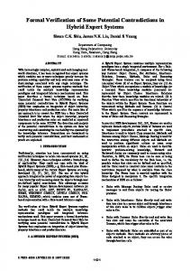
Fig. 1. Results of validated simulation: y2 w.r.t. y1 . with {y(t; y0 ) : ∀y0 ⊆ [y0 ]} ⊆ [y], and  n IR e  7→ IR R: t, t → [e y]

(4)

with {y(t; y0 ) : ∀y0 ∈ [y0 ] ∧ ∀t ∈ [t, t]} ⊆ [e y]. Function R, defined in (3), is obtained by new applications of validated integration method starting from [yk ] at tk , and e defined in finishing at t with tk < t < tk+1 . Function R, (4), is obtained with the union of [e yk ] with k = a, . . . , b and ta < t < t < tb . These functions are then strictly conservative. e define two interval More abstractly, the functions R and R enclosures of the solution function of differential equations defined in Equation (2). Example 3: We consider an Initial Value Problem based on the following constrained differential algebraic equation      y˙1 = −y3 y2 − (1 + y3 )x1     F : y˙2 = y3 y1 − (1 + y3 )x2        y˙3 = 1  ( (5)  0 = (y1 − x2 )/5 − cos(y32 /2)   G:    0 = (y2 − x1 )/5 − sin(y32 /2)       H : 0 = x21 + x22 − 1 and the initial values y(0) = (5, 1, 0) and x(0) = (−1, 0). Interesting variables are y1 and y2 , the states of the system. A picture of the result of validated simulation is given in Figure 1 and Figure 2. It follows an example of the use of the functions providing e enclosures at given time R(t) and R([t]): R(1.1) = ([5.001, 5.006]; [3.294, 3.299]; [1.099, 1.100]) e R([0.7, 0.8]) = ([5.463, 5.495]; [1.975, 2.270]; [0.699, 0.800]) The problem given by Equation (5) has a known exact solution which is  2   y1 = sin(t) + 5 cos(t /2) y(t) = y2 = cos(t) + 5 sin(t2 /2) .   y3 = t • •

Journal of Software Engineering for Robotics 8(1), December 2017

82

•

•

•

Fig. 2. Results of validated simulation: y2 w.r.t. time.

If we compute the previous enclosures with the exact solution (by combining interval arithmetic with bisection method to obtain sharp results), we find: • y(1.1) = ([5.003, 5.003]; [3.297, 3.297]; [1.1]) • y([0.7, 0.8]) = ([5.464, 5.494]; [1.977, 2.269]; [0.7, 0.8]) e The enclosure property of R(t) and R(t) is then verified. 

3

CSP

WITH

D IFFERENTIALS C ONSTRAINTS

Constraint Satisfaction Differential Problems (CSDP) extending the definition of NCSP have been defined in [7] by adding new variables to represent time derivative, i.e., dy dt and a new = F (y, t), or a more kind of constraints of the form dy dt complex differential equation as given in Equation (2). The main drawback of CSDPs is that temporal properties cannot be encoded because the time variable t is not a variable of the problem. So, for example, the property “for all t in [0, 10], the system does not collide with an obstacle” cannot be represented as a CSDP in an obvious manner. The work [8] considers differential equations as an implicit definition of temporal functions. In consequences, considering only solution function Φ of differential equations makes an easy embedding of differential equations into NCSP framework. Unfortunately, NCSPs naturally express existential probVn lems, i.e., problems of the form ∃x ∈ [x], f (x) = i=1 i Vm 0 ∧ i=1 gi (x) 6 0. While this approach is appealing to simply embed differential equations into constraint programming framework, it is also unable to express constraints where the time variable is a variable of the problem. In both previous work [7] and [8], the main drawback is the lack of quantification on variables. A proposition of extension of these approaches to cope with this limitation is the main contribution of the paper. In order to be able to define a CSDP which can answer a question of the type “Will the system collide with an obstacle before ten seconds?”, we propose a new definition of CSDP which mainly introduces quantification over variables. Definition 2 (QCSDP): Let S be a differential system as defined in (2) and tend ∈ R+ the time limit of the problem handled. A QCSDP is a CSP defined by:

a set of variables V including at least the time variable t, a vector y0 of dimension n representing the initial state-space of S, variables associated to the parameters p, variables representing the control input u of S. We represent these variables by the vector v; an initial domain D containing at least [0, tend ] for time t, the initial domain Y0 of initial condition y0 , U for control input u, and P for parameters p; a set of constraints C = {c1 , . . . , ce } composed of predicates over sets, that is, constraints of the form: ci (v) ≡ Qv ∈ Di .fi (v)  A,

∀1 6 i 6 e,

with Q ∈ {∃, ∀}, fi : ℘(R|V| ) → ℘(Rq ) stands for nonlinear arithmetic expressions defined over variables v and solution of differential system S, y(t; y0 , p, u) ≡ y(v). The operator  denotes {⊂ , ⊃ , ∩=∅ , ∩6=∅ }, i.e., the setbased operations, and the set A ⊂ Rq where q > 0. Note that ∩=∅ stands for the predicate f (v) ∩ A = ∅ and ∩6=∅ stands for the predicate f (v) ∩ A = 6 ∅. ℘(E) denotes the power-set of the set E, while |E| denotes the cardinality of E. Note that in Definition 2, the constraints are expressed with set-based operator instead of equalities and inequalities to simplify the notations despite the complete equivalence with equalities and inequalities. Moreover, set-based operations will emphasize, in Section 4, one important difficulty due to the representation of sets with respect to the correctness of the proposed approach. As the QCSDP over sets is not computable in general, a set abstraction has to be used. Moreover, solving arbitrary quantified constraints over reals is a hard problem hence we focus on certain classes of problems related to the robotic domain. In particular, three main classes are considered. Problem 1 deals with the design of robot platform or control algorithms and for example is treated with a CSP approach in [19] or in [20] (the latter is recalled in Section 5). Problem 2 deals with the design of robust control algorithms. It is the case study of Section 6 and it has been considered in the context of non-linear sampled switch systems in [21]. Problem 3 consists in finding the subset of initial states such that there exists at least one evolution ”viable”, in the sense that at each time, the state of the evolution remains confined to the viability kernel [22]. The problem of viability kernel computation has been considered by the help of our method in [23]. Problem 1 (Appropriate design): A parametric dynamics of a robot described by a differential system is considered, the parameters represent some possible choices in the characteristics of the robot such as its dimension, the power of the engine and so on. An appropriate design problem aims at finding a value of the parameters such that a set of functional requirements is fulfill. In other words, QCSDP problems are made of constraints over variables p, u and y0 based on quantification ∃p, ∀u, ∀y0 , and some temporal constraints (see Section 4).

J. Alexandre dit Sandretto et al./ Preparation of Papers for Journal of Software Engineering for Robotics

Problem 2 (Control synthesis): A parametric dynamics of a robot described by a differential system is considered, the parameters represent perturbation. A control synthesis problem aims at finding value of the control u such that some requirements are fulfill taking into account all possible perturbations. In other words, QCSDP problems are made of constraints over variables p, u and y0 based on quantification ∃u, ∀p, ∀y0 , and some temporal constraints (see Section 4). Problem 3 (Viability kernel): A parametric dynamics of a robot described by a differential system is considered, the parameters represent perturbation. A viability kernel problem aims at finding initial values of the system such that there exists at least one evolution remaining into the viability kernel taking into account all possible perturbations. In other words, QCSDP problems are made of constraints over variables p, u and y0 based on quantification ∃y0 , ∀p, ∃u, and some temporal constraints (see Section 4). Note that it is also possible to add a cost function in the Definition 2, and hence consider constraint optimization problems. The considered problem is then a Quantified Constraint Satisfaction Differential Optimization Problem, and defined as follows. Definition 3 (QCSDOP): A Quantified Constraint Satisfaction Differential Optimization Problem involves in addition an objective function Q(v1 , . . . , vn ) that has to be maximized or minimized over the set of all feasible solutions of a QCSDP. As differential equations are seamlessly integrated into QCSP framework, dealing with cost functions is straightforward following classical techniques [24].

4

R EASONING U NDER S ET A BSTRACTION

In Definition 2, QCSDPs are defined over sets of values and hence they are not computable. Abstraction with boxes is considered in this section. By denoting α() the box abstraction, the constraints of QCSDP presented above becomes: α(ci (v)) ≡ α(Qv ∈ Di .fi (v)  A)

(6)

≡ Qv ∈ [di ].α(fi (v)  A)

(7)

≡ Qv ∈ [di ].[fi ](v)α(A) .

(8)

From Equation (6) to Equation (7), abstraction consists on an over-approximation of the domain of variables. Then, from Equation (7) to Equation (8), the interval enclosure is used as an abstraction of function f . It means that only enclosure of the solution of differential equations is considered, even if an inner approximation could be available. Indeed, enclosure is mainly favored because the approach presented in this paper is oriented to safety problems and not to liveness. Abstraction α(A) is not distributive in a safe manner. Applied to the set A, the function α ∈ {Hull, Int} stands for an interval abstraction function which maps a set A to a set of boxes. Hull(A) stands for the interval over-approximation of the set A while Int(A) stands for an interval representation (a single

83

interval or a paving) of an under-approximation of the set A. For soundness, Hull(A) encloses the hull of A, and Int(A) is included in the interior of A. By an abuse of notation,  in Definition 4 will denote the abstraction of the set-theoretic operator  given in Definition 2 but it is important to keep in mind that the implementation is strongly dependent on the abstraction of the set A. The possible operations are gathered in the Table 1. Due to the abstraction, all these operators are weak. Nevertheless, some results after abstraction imply the original logic formula. In Table 1, question mark “?” means that neither true nor false implies a guaranteed result on the original logic formula. On the contrary, true means that if the abstract formula is valid, then the original one is valid, i.e., [f ](v) ⊂ Int(A) ⇒ f (v) ⊂ A. In the same way, false means that if the abstract formula is not valid, then the original one is not valid, i.e., ¬([f ](v) ∩6=∅ Hull(A)) ⇒ ¬(f (v) ∩6=∅ A). Abstraction function α(A) can be distribute into α()α(A) by following carefully the results presented in Table 1. Finally, we propose the Box-QCSDP formalism, which is a QCSP where sets are represented by boxes and is formally defined in Definition 4. It mainly introduces two abstractions: the abstraction of the solution of differential systems as defined in (2); and the abstraction of constraints ci , in particular, the abstraction of the set A. The first and major abstraction allows us to manage with the differential system in a CSDP. It is performed by a validated simulation method as described in 2.3. This approach provides to us two abstraction functions guaranteed to enclose all the behaviors of the differential system. The second abstraction is done to be able to handle the sets by an outer or an inner approximation, depending on the associated logic operation. In order to correctly translate a satisfaction problem, these capabilities offered by QCSDP have to be used in the right way. Definition 4 (Box-QCSDP): Let S be a differential system as defined in (2) and tend ∈ R+ the time limit of the problem handled. A Box-QCSDP is defined by: • a set of variables V including at least the time variable t, a vector y0 of dimension n representing the initial state-space of S, variables associated to the parameters p, variables representing the control input u of S. We represent these variables by the vector v; TABLE 1 Available operations

α(f )

[f ]

⊂ ⊃ ∩=∅ ∩6=∅

α(A) Int(A) Hull(A) true ? false ? ? true ? false

Journal of Software Engineering for Robotics 8(1), December 2017

84

•

•

TABLE 2 Available operations

an initial box domain [d] containing at least [0, tend ] for time t, the initial box [y0 ] of initial condition y0 , a box [u] for control input u, and a box [p] for parameters p; a set of constraints C = {c1 , . . . , ce } composed of predicates over sets, that is, constraints of the form ci ≡ Qv ∈ [di ].[fi ](v)α (A) ,

Verbal property Stay in A Stay in A till τ One in A Has crossed A Go out A Has reached A Finish in A

∀1 6 i 6 e,

with Q ∈ {∃, ∀}, [fi ] : IR|V| → IRq stands for an inclusion function of non-linear arithmetic expressions defined over variables v and an interval enclosure of the solution of differential system S, [y](t; [y0 ], [p], [u]). The set theory based operations are expressed by  ∈ {⊂, ⊃, ∩=∅ , ∩6=∅ } and a set A ⊂ Rq where q > 0. The function α(A) maps a part of logic operations into abstract ones, following Table 1. Definition 4 is very dependent of the implementation. The following remarks give some insight to produce safe results. Remark 1: If a validated simulation cannot reach tend and e fails at t = tfail then R(t) = [−∞, ∞], for all t > tfail . Hence the enclosure of [y](t; [y0 ], [p], [u]) is always correct and respects the contractor definition. Remark 2: Solutions of differential equations need to be pre-computed to obtain our abstraction functions R(t) and e R([t]). If the parameters or control inputs involved in the definition of the differential equation is reduced by the CSDP solver, then the abstraction functions need to be computed again. It is a part of the propagation algorithm of a CSP. QCSDP, see Definition 2, allows one to describe a complex satisfaction problem in order to reason about a system defined by a differential equation. Nevertheless, a definition of the temporal constraints has not been done yet, it is the purpose of the end of this section. We consider the main interesting properties for robotic applications, by providing verbal operators in the sense of “system has the property of”, such as “stay in till”. By convention, these Boolean operations provide a guaranteed true answer. It means that “true” is proven while “false” means “uncertain” due to the abstraction of boxes. In table 2, the different available verbal operators and their Box-QCSDP translation are gathered. Despite this list of specifications is limited it emphasizes the main difficulty to reason on abstraction of the behaviors of robots. From table 2 and due to the abstraction, “Go out” is not equivalent to ¬(“Stay in”). Operators “Has reached” and “Has crossed” are poor tests (true means uncertain). They are equivalent but the validity of “Has reached” at the end of a simulation implies a notion of stability. On the other hand, the negation of these latter operators are strong and are useful to speed up a Box-QCSDP solver. Following the same generalization than for Constraint Optimization Problems based on CSP, a cost function can be added to Box-QCSDP to perform optimization. Definition 5 (Optimization on Box-QCSDP): A Box-Quantified Constraint Optimization Differential Problem involves in

CSDP translation ∀t ∈ [0, tend ], R(t) ⊆ Int(A) ∀t ∈ [0, τ ], R(t) ⊆ Int(A) ∃t ∈ [0, tend ], R(t) ⊆ Int(A) ∃t ∈ [0, tend ], R(t) ∩ Hull(A) 6= ∅ ∃t ∈ [0, tend ], R(t) ∩ Hull(A) = ∅ R(tend ) ∩ Hull(A) 6= ∅ R(tend ) ⊂ Int(A)

addition of a Box-QCSDP an objective function Q(v1 , . . . , vn ) that has to be maximized or minimized over the set of all feasible solutions. The details on algorithms to solve optimization problems is out of the scope of this paper, but they are the same than the ones used for CSP [24]. Box-QCSDP and this list of specifications have been implemented in a library named DynIBEX1 [25]. To obtain a solution which is safe (e.g.w.r.t. obstacles), it is important to obtain an inner approximation of the Box-QCSDP solution set. In this case, we consider that the problem contains only hard constraints (different than soft ones, which can be violated). This consideration is general in our approach and we are looking only for inner solution of hard constraints. The inner solutions are obtained with the algorithm given in Algorithm 1, and gathered in Sacc . Algorithm 1 A generic Branch&Prune Require: S = {[v]}, Sacc = ∅, Srej = ∅, Sunc = ∅ while S 6= ∅ do Pop a [v]current from S if c1 ([v]current ) AND . . . AND ce ([v]current ) then Push [v]current in Sacc else if NOT c1 ([v]current ) OR . . . OR NOT ce ([v]current ) then Push [v]current in Srej else if Width([v]current ) > ε then ([v]left , [v]right ) = Bisect([v]current ) Push [v]left in S Push [v]right in S else Push [v]current in Sunc end if end while

5

C ASE S TUDY 1:

CONTROLLER SYNTHESIS

We exploit the Box-QCSDP formalism to synthesize the parameters of a Proportional-Integrator (PI) controller in the case of a cruise-control system [20]. 1. http://perso.ensta-paristech.fr/∼chapoutot/dynibex/

J. Alexandre dit Sandretto et al./ Preparation of Papers for Journal of Software Engineering for Robotics

85

The vehicle to be controlled has a mass m, a velocity v, and is acted by a control force u representing the force generated at the road/tire interface. It is assumed that control on u can be done directly. In this form is also considered that the resisting forces bv of the rolling resistance and wind drag vary linearly with v and act in the opposite direction of the vehicle’s motion. Air particles flow over the hood of the vehicle causing the aerodynamic drag which can be modeled by Fdrag = 0.5ρCdAv 2

(9)

where ρ is the density of air, CdA is the coefficient of drag for the vehicle times the reference area. Here the density of the air is considered equal to 1.2041 kg/m3 obtained with a temperature of 20◦ C and an atmospheric pressure of 101kPa. The vehicle system is then described by the ODE (u − bv − 0.5ρCdAv 2 ) (10) m The solution of Equation (10) is denoted by v(t; v0 , u). The setpoint vset on the speed is defined and corresponds to the particular velocity we want for the vehicle. So the error e(t) = vset − v and the force needed to make the vehicle go with a velocity in vset is given by the PI Z u = Kp (vset − v) + Ki (vset − v)ds. (11)

Fig. 3. Paving of PI parameters Kp × Ki for the non-linear cruise-controller – in blue accepted and in red rejected

v˙ =

Finaly, the result in term of response of the system is given in Figure 4. On this picture, one can see that the constraints are validated.

The synthesis of PI controller consists on the computation of a paving of the set of validated PI parameters Kp and Ki . For that, we simulate the dynamical system controlled by a PI whose parameters are in an interval. A PI controller defined by (Kp , Ki ) is validated if it satisfies safety (limited overshoot), convergence to the setpoint and stability. These properties can be translated into constraints:   v(t; v0 , Kp , Ki ) ∈ [vmin , vmax ], ∀t ∈ [0, tend ], (12) v(tend ; v0 , Kp , Ki ) ∈ [vset − α, vset + α],   v(t ˙ end ; v0 , Kp , Ki ) ∈ [−, ],  > 0. These constraints can be translated into our formalism of Box-QCSDP: V = {t, v0 , Kp , Ki } ,

Fig. 4. Response of controller for non-linear plant v(t) w.r.t. t, with parameters validated (Kp = 1400 and Ki = 35).

D = {[t] = [0, tend ], [v0 ] = [0, 0.1], [Kp ] = [0, 4000], [Ki ] = [0, 120]} , C={ c1 = ∀t ∈ [t] · [v](t; [v0 ], Kp , Ki ) ⊂ [vmin , vmax ],

(13)

c2 = [v](tend ; [v0 ], Kp , Ki ) ⊂ vset + [−α, α], c3 = [v](t ˙ end ; [v0 ], Kp , Ki ) ⊂ [−, ] } . The algorithm 1 can be used to solve the Box-QCSDP (13) (with b = 50, 0.5ρCdAv 2 = 0.4, tend = 10, vset = 10, m = [990, 1010], α = 0.02 and  = 0.2), and the results are given in Figure 3.

6

C ASE S TUDY 2: R OBOT PATH P LANNING

We present an application of Box-QCSDP based on the algorithm Box-RRT defined in [26] which aims at producing a robust path for a car-like vehicle while avoiding obstacles. The dynamic model of the car is defined by  x˙ = v cos(θ)    y˙ = v sin(θ) . (14)    θ˙ = v tan (δ + ε) L

Journal of Software Engineering for Robotics 8(1), December 2017

86

Fig. 6. Two results of Box-RRT, an unlucky try (left) and a lucky try (right)

Fig. 5. Results of Box-RRT

The state of the car is defined by the car position (x, y) and its heading θ. L is the distance between the front and rear wheels. There are two control inputs v for the longitudinal speed and δ ∈ [δmin , δmax ] for the steering angle. The noise element ε = [−0.001, 0.001] stands for the steering angle imprecision. A second source of uncertainties is the initial position of the vehicle. We denote by car(t; s0 ) the solution of Equation (14) and by [car](t; s0 ) its interval enclosure produce by guaranteed integration methods. We denote by s0 = (x0 , y0 , θ0 ) and [s0 ] = [x0 ] × [y0 ] × [θ0 ] the state variables and the initial conditions. We denote by [sf ] the targeted state-space. Box-RRT algorithm extends Rapid Random Tree (RRT) algorithm with interval analysis tools. A brief recall of the BoxRRT algorithm is given before introducing our formalization with Box-QCSDP. From a map, denoted by Map, represented by a paving, i.e., a set of non-overlapping boxes and from a list of obstacles, denoted by La , Box-RRT looks for a safe path between [s0 ] and [sf ], avoiding all obstacles in La and staying in Map. To do this, a tree T of possible paths is generated from a random walk inside the state-space represented by a paving. Box-RRT is an iterative algorithm which mainly follows three steps until [sf ] is reached i) pick a random state [srandom ], ii) find the closest state of [srandom ] in the tree T named [snearest ], iii) pick a control u and compute [snew ] which is the final state of the trajectory starting from [snearest ] with the control u. If this trajectory reaches an obstacle, an other state is chosen. Otherwise if [snew ] ⊂ [sf ] then a path is found and the algorithm terminates. Otherwise, the target

[sf ] has not been reached and [snew ] is a possible safe state being on the path to reach the target [sf ]. Hence, [snew ] is added as a new node in T and the exploration of the state-space continues. In Box-RRT algorithm, Step 3 is a Box-QSCDP. In particular, there are several constraints that must be taken into account while the path is generated. First, the path generation works on a finite dimension map and so trajectories must stay inside this map. Obviously, a constraint expressing the avoidance of obstacles shall be considered. An other constraint has to be defined to detect when a trajectory reaches the targeted region of the state-space. In consequence, the path generation is translated into Box-QCSDP which is defined in Equation (15). Note that this Box-QCSDP has to be solved at each iteration of the Box-RRT algorithm until a path has been found. V = {t, x0 , y0 , θ0 , v, δ} , D = {[t] = [0, 1], [x0 ] = [0.0, 0.3], [y0 ] = [0.0, 0.3], [θ0 ] = [0.0]} , C={ c1 = ∀s0 ∈ [s0 ], ∀t ∈ [t] · [car](t; s0 ) ⊂ Map, c2 = ∀s0 ∈ [s0 ], ∀t ∈ [t], ∀sa ∈ [La ] · [car](t; s0 ) ∩6=∅ sa , c3 = ∀s0 ∈ [s0 ], ∃t ∈ [t] · [car](t; s0 ) ⊂ [sf ] } . (15) In Equation (15), the constraint c1 states that the trajectory [car](t) from [snearest ] to [snew ] has to stay inside the map Map. The constraint c2 states that the trajectory [car](t) shall not intersect an obstacle and finally the constraint c3 states that a path is found if one state of trajectory is included into [sf ]. An example of the exploration of the state-space produced by the Box-RRT algorithm is given in Figure 5. The red squares stand for obstacles while the blue square represents [sf ]. The small black square in the center of the figure is [s0 ] while the black square inside [sf ] is the final state of the trajectory reaching the target.

J. Alexandre dit Sandretto et al./ Preparation of Papers for Journal of Software Engineering for Robotics

On a laptop, one subpath takes around 25 milliseconds to be tested. On one hundred tentatives, the quickest one needed 26 subpaths to achieve the complete path and the slowest one needed 2532 subpaths (the median is equal to 394). Two experimentations, one “unlucky” and one “lucky” are given in Figure 6.

7

R EFERENCES

[2] [3]

[4] [5]

[7] [8]

C ONCLUSION

In this paper, we presented a framework for the formal verification of robotic behaviors in presence of uncertainties. Based on the constraint satisfaction problem formalism and with the help of interval tools such as interval arithmetic and the validated integration of differential equations, a method to verify the safety, in a guaranteed manner, has been developed. Our approach mainly exploits box abstraction of uncertainties, sets, functions and differential equations. Box abstraction is a very powerful approach to deal with uncertainties and, more particularly, with differential equations. Nevertheless, this abstraction introduces another difficulty, which is the handling of logic formula, because some logic operators become weak. We carefully analyzed available operators and a new formalism called Box-QCSDP has been finally presented. The problem of controller synthesis has been translated into BoxQCSDP formalism and solved. Then a well known problem, the robot path planning, has been studied under the formalism of Box-QCSDP. An algorithm based on Rapid-exploring Random Tree has been defined including constraints (obstacles and objectives) and solved with our method. The resulting path is guaranteed by construction, considering the robot dynamics, which is an interesting improvement of classical path planners. To conclude, we presented in this paper a new formalism that allows one to solve complex problems linking dynamical systems and temporal logic, in a validated way. In a future work, we plan to incorporate the framework of Box-QCSDP into a higher level of problem solver such as SAT solvers or model checkers. Other applications in robotics, using constraint programming and optimization procedure, are ongoing such as optimal control or optimal motion planning.

[1]

[6]

M. Rueher, “Solving continuous constraint systems,” in International Conference on Computer Graphics and Artificial Intelligence, 2005. 1, 2.2 N. S. Nedialkov, K. Jackson, and G. Corliss, “Validated solutions of initial value problems for ordinary differential equations,” Appl. Math. and Comp., vol. 105, no. 1, pp. 21 – 68, 1999. 1, 2.3, 2.3 A. Rauh, M. Brill, and C. G¨uNther, “A novel interval arithmetic approach for solving differential-algebraic equations with ValEncIAIVP,” International Journal of Applied Mathematics and Computer Science, vol. 19, no. 3, pp. 381–397, 2009. 1 J. Alexandre dit Sandretto and A. Chapoutot, “Validated Explicit and Implicit Runge-Kutta Methods,” Reliable Computing electronic edition, vol. 22, 2016. 1, 2.3, 2.3, 2.3 ——, “Validated Simulation of Differential Algebraic Equations with Runge-Kutta Methods,” Reliable Computing electronic edition, vol. 22, 2016. 1, 2.3, 2.3, 2.3, 2.3

[9]

[10] [11]

[12]

[13] [14] [15] [16] [17] [18] [19] [20]

[21]

[22] [23]

[24] [25] [26]

87

M. Janssen, Y. Deville, and P. Van Hentenryck, “Multistep filtering operators for ordinary differential equations,” in Principles and Practice of Constraint Programming, ser. Lecture Notes in Computer Science. Springer, 1999, vol. 1713, pp. 246–260. 1 J. Cruz and P. Barahona, “Constraint reasoning over differential equations,” Applied Numerical Analysis and Computational Mathematics, vol. 1, no. 1, pp. 140–154, 2004. 1, 3 A. Goldsztejn, O. Mullier, D. Eveillard, and H. Hosobe, “Including ordinary differential equations based constraints in the standard CP framework,” in Principles and Practice of Constraint Programming, ser. Lecture Notes in Computer Science. Springer, 2010, vol. 6308, pp. 221–235. 1, 3 B. Hoxha and G. E. Fainekos, “Planning in dynamic environments through temporal logic monitoring,” in AAAI Workshop: Planning for Hybrid Systems, ser. AAAI Workshops, vol. WS-16-12. AAAI Press, 2016. 1 J. Liu, N. Ozay, U. Topcu, and R. M. Murray, “Synthesis of reactive switching protocols from temporal logic specifications,” Automatic Control, IEEE Transactions on, vol. 58, no. 7, pp. 1771–1785, 2013. 1 A. Eggers, M. Fr¨anzle, and C. Herde, “SAT modulo ODE: A direct SAT approach to hybrid systems,” in Automated Technology for Verification and Analysis, ser. Lecture Notes in Computer Science. Springer, 2008, vol. 5311, pp. 171–185. 1 S. Gao, S. Kong, and E. M. Clarke, “dReal: An SMT solver for nonlinear theories over the reals,” in International Conference on Automated Deduction, ser. Lecture Notes in Computer Science, vol. 7898. Springer, 2013, pp. 208–214. 1 R. E. Moore, Interval Analysis, ser. Series in Automatic Computation. Prentice Hall, 1966. 2.1 L. Jaulin, M. Kieffer, O. Didrit, and E. Walter, Applied Interval Analysis. Springer, 2001. 2.1, 2.2.1 Y. Lebbah and O. Lhomme, “Accelerating filtering techniques for numeric CSPs,” Journal on Artificial Intelligence, vol. 139, no. 1, pp. 109 – 132, 2002. 2.2 F. Benhamou, D. McAllester, and P. Van Hentenryck, “Clp (intervals) revisited,” Providence, RI, USA, Tech. Rep., 1994. 2.2 G. Chabert and L. Jaulin, “Contractor programming,” Artificial Intelligence, vol. 173, no. 11, pp. 1079–1100, 2009. 2.2 O. Lhomme, “Consistency techniques for numeric CSPs,” in International joint conference on Artifical intelligence, 1993, pp. 232–238. 2 J. Alexandre dit Sandretto, D. Piccani de Souza, and A. Chapoutot, “Appropriate design guided by simulation: An hovercraft application,” in Model-Driven Robot Software Engineering. ACM, 2016. 3 J. Alexandre dit Sandretto, A. Chapoutot, and O. Mullier, “Tuning PI controller in non-linear uncertain closed-loop systems with interval analysis,” in Synthesis of Complex Parameters, ser. OpenAccess Series in Informatics (OASIcs), vol. 44. Schloss Dagstuhl–Leibniz-Zentrum fuer Informatik, 2015, pp. 91–102. 3, 5 A. Le Coent, J. Alexandre dit Sandretto, A. Chapoutot, and L. Fribourg, “Control of Nonlinear Switched Systems Based on Validated Simulation,” in Symbolic and Numerical Methods for Reachability Analysis, Vienna, Austria, 2016. 3 J.-P. Aubin, “A survey of viability theory,” SIAM Journal on Control and Optimization, vol. 28, no. 4, pp. 749–788, 1990. 3 D. Monnet, L. Jaulin, J. Ninin, J. Alexandre dit Sandretto, and A. Chapoutot, “Viability kernel computation based on interval methods,” in Small Workshop on Interval Methods, Prague, Czech Republic, 2015. 3 E. R. Hansen, Global Optimization Using Interval Analysis, 2nd ed. CRC Press, 2003. 3, 4 J. Alexandre dit Sandretto and A. Chapoutot, “DynBEX: a Differential Constraint Library for Studying Dynamical Systems (Poster),” in Conference on Hybrid Systems: Computation and Control, 2016. 4 R. Pepy, M. Kieffer, and E. Walter, “Reliable robust path planning with application to mobile robots,” International Journal of Applied Mathematics and Computer Science, vol. 19, no. 3, pp. 413–424, 2009. 6

88

Julien Alexandre dit Sandretto is a research associate in the Safety and Reliability of Software team at ENSTA ParisTech, Palaiseau, France. He is also associate member of the Cosynus team, part of the LIX laboratory at ´ Ecole Polytechnique. He received the Bachelor degree in Applied Mathematics and Computer Science from the University Joseph Fourier, Grenoble, France, in 2002 and the Eng. degree in Industrial Computing and Instrumentation from Polytechnic school of Grenoble, France, in 2006. In 2013, he obtained his Ph.D. degree in Computer Science from University of Nice-Sophia Antipolis, France. His research interests deal with verification methods in presence of uncertainties. He currently focuses on parameter identification, simulation, modeling and control problems for cyber-physical systems.

Journal of Software Engineering for Robotics 8(1), December 2017

Alexandre Chapoutot is an Associated professor at ENSTA ParisTech since 2010. He received his Ph.D. in Computer Science from Ecole polytechnique in 2008 for his work on static analysis by abstract interpretation of hybrid systems. He received his master degree in Computer Science from University Pierre et Marie Curie (UPMC) in 2005. He worked as a research and teaching assistant at University Pierre et Marie Curie, at LIP6, where he studied the accuracy of floatingpoint computations in programs. His research activities are mainly focused on the definition and the application of set-based methods, for the analysis and the verification of properties of cyber-physical systems. He is also interested in the analysis and the improvement of floating-point accuracy in programs.

olivier Mullier is a Postdoctoral Researcher at ENSTA Paristech, France. He is a member of the computer science and system engineering unit (http://u2is.ensta-paristech.fr) and involved in the DGA/MRIS project on Operational security in robotic systems. His research interests include formal methods in the context of cyber physical systems using set-membership computation. He received his PhD in Computer Science ´ from Ecole Polytechnique, France in 2014. He has studied Computer Science in optimization and Operation research in university of Nantes where he has received his Master’s degree.