Foveated self-similarity in nonlocal image
ltering
Alessandro Foia and Giacomo Boracchib a Department
of Signal Processing, Tampere University of Technology, P.O. Box 553, 33101 Tampere, Finland b Dipartimento di Elettronica e Informazione, Politecnico di Milano, via G. Ponzio, 34/5, 20133 Milano, Italy ABSTRACT
Nonlocal image …lters suppress noise and other distortions by searching for similar patches at di¤erent locations within the image, thus exploiting the self-similarity present in natural images. This similarity is typically assessed by a windowed distance of the patches pixels. Inspired by the human visual system, we introduce a patch foveation operator and measure patch similarity through a foveated distance, where each patch is blurred with spatially variant point-spread functions having standard deviation increasing with the spatial distance from the patch center. In this way, we install a di¤erent form of self-similarity in images: the foveated self-similarity. We consider the Nonlocal Means algorithm (NL-means) for the removal of additive white Gaussian noise as a simple prototype of nonlocal image …ltering and derive an explicit construction of its corresponding foveation operator, thus yielding the Foveated NL-means algorithm. Our analysis and experimental study show that, to the purpose of image denoising, the foveated self-similarity can be a far more e¤ective regularity assumption than the conventional windowed self-similarity. In the comparison with NL-means, the proposed foveated algorithm achieves a substantial improvement in denoising quality, according to both objective criteria and visual appearance, particularly due to better contrast and sharpness. Moreover, foveation is introduced at a negligible cost in terms of computational complexity. Keywords: nonlocal image modeling, foveation, image denoising, human visual system, self-similarity.
1. INTRODUCTION We investigate the connections between the human visual system (HVS) and nonlocal algorithms in imaging. Speci…cally, we focus on the role of foveation in nonlocal image …ltering. As a simple prototype of nonlocal …lters for images, we consider the Nonlocal Means (NL-means) algorithm1 for removal of additive white Gaussian noise. Its basic idea is to build a pointwise estimate of the image where each pixel is obtained as a weighted average of pixels that lie at the center of patches (i.e. neighborhoods, regions) that are similar to the patch centered at the estimated pixel. The estimates are nonlocal since similar patches can be found at di¤erent locations within the image and, in principle, the averages can be calculated over all pixels of the image. The pairwise similarity between patches (often referred to as nonlocal self-similarity) determines the weights used in the averaging, so that the higher is the similarity the larger are the weights. In NL-means, the similarity between di¤erent patches is measured through the windowed quadratic distance of the gray-level intensities (i.e. windowed photometric distance), where the window function decays smoothly to zero as we move away from center of the corresponding patch. In this work, we replace such windowed distance with a foveated distance: instead of multiplying the photometric di¤erences against a window function, we compute the distance between foveated patches, i.e. patches blurred by point-spread functions having increasing standard deviation (thus increasing spread) as the spatial distance from the center of the patch grows. If we treat the point to be estimated as a …xation point, this foveated distance mimics the inability of the HVS to perceive details at the periphery of the center of attention. Our analysis and experimental study show that utilizing a foveated self-similarity instead of the conventional windowed self-similarity leads to an improvement in the resulting image estimate, according both to objective criteria and visual appearance, particularly due to better contrast and sharpness. This work was supported by the Academy of Finland (project no. 213462, Finnish Programme for Centres of Excellence in Research 2006-2011, project no. 129118, Postdoctoral Researcher’s Project 2009-2011, and project no. 252547, Academy Research Fellow 2011-2016). E-mail contacts: alessandro.foi@tut.…,
[email protected].
2. OBSERVATION MODEL We consider observations as noisy grayscale images z : X ! R that can be modeled as z (x) = y (x) + (x) ,
Z2 ,
x2X
(1)
where X Z2 is the image domain, which is assumed a regular pixel grid, y : X ! R is the unknown original image, and : X ! R is i.i.d. Gaussian white noise, ( ) N 0; 2 . The purpose of any denoising algorithm is to provide an estimate y^ of the original image y. Image patches play a central role and, for the sake of clarity, we introduce a speci…c notation for them. Let U Z2 be a neighborhood centered at the origin; we de…ne a patch centered at a pixel x 2 X in the observation z as zx (u) = z (u + x) ; u 2 U . Similarly, we de…ne the noise-free patches as
yx (u) = y (u + x) ;
u 2 U.
3. NONLOCAL MEANS The use of nonlocal self-similarity in image processing gained signi…cance with the fractal models of natural images (e.g.,2 ). For the speci…c task of noise attenuation, nonlocality has been initially considered in,3 and later developed in the NL-means algorithm,1, 4 representing a breakthrough in image denoising and inspiring several powerful algorithms in the following years (e.g., BM3D5 or SAFIR6 ). Nonlocal …ltering and, more generally, patch-based algorithms lately became established paradigms, which are successfully applied to a broad range of imaging applications. For a comprehensive overview on modern denoising approaches and algorithms we refer the reader to,7 while in the present paper, for the sake of simplicity and to elucidate our contribution, we restrict our attention to the NL-means algorithm. In its basic implementation, the NL-means admits the following simple and elegant formulation. The denoised image y^ consists in a weighted average of potentially all the image pixels, i.e. X y^(x1 ) = w (x1 ; x2 ) z(x2 ); 8x1 2 X; (2) x2 2X
where fw(x1 ; x2 )gx2 2X is the set of adaptive weights that characterize the pixel x1 , which are positive and sum to one. Each weight w(x1 ; x2 ) is determined by the similarity between the two patches zx1 and zx2 , as w (x1 ; x2 ) = e
d(x1 ;x2 ) h2
=
P
e
d(x1 ;x) h2
;
(3)
x2X
where d (x1 ; x2 ) is a distance measure between image patches centered at x1 and x2 , and h > 0 is a …ltering parameter controlling the decay of the exponential function. Equation (3) assigns larger weights to the terms z ( ) in (2) that correspond to pixels belonging to similar patches (i.e. where the distance between patches d(x1 ; x2 ) is small), regardless of their location within the image. This motivates the nonlocal denomination of the algorithm. Thanks to such a weighting mechanism, the NL-means enforces the self-similarity of natural images, which turns out to be an e¤ective regularity prior for suppressing the noise. The distance d is de…ned as a windowed quadratic distance between patches, i.e. X p p 2 2 2 d(x1 ; x2 ) = zx1 k zx2 k = (zx1 zx2 ) k = (z(u + x1 ) z(u + x2 )) k (u) ; 2
1
(4)
u2U
being k a non-negative windowing kernel de…ned over U , which allows to adjust the contribution of each term depending on the position of u with respect to the patch center. Typically, k is rotational symmetric and the weights k(u) are determined by the spatial distance from the center. In the original formulation of NL-means,1 the authors suggest using a Gaussian function (with …xed standard deviation) as windowing kernel k, while in practice various windowing kernels having maximum at the patch center are also adopted.8 In practice, due to computational aspects, for each x1 , only pixels x2 belonging to a limited search window around x1 are considered for the sum (2).
The motivating idea of using (4) is very practical: the similarity between y (x1 ) and y (x2 ) (which are not available) can be assessed by computing the similarity of the corresponding noisy patches, i.e., zx1 and zx2 . The noise in‡uence is thus reduced by evaluating the similarity over patches, and the decay of k re‡ects to which extent the similarity between y (u+x1 ) and y (u+x2 ) at each u 6= 0 implicates the similarity between y (x1 ) and y (x2 ). 2
Given a pair of arbitrary noise-free patches yx1 ; yx2 , the term (zx1 zx2 ) (u) follows a non-central chi2 squared distribution having mean (yx1 yx2 ) (u) + 2 2 , thus, we can easily compute the expectation of the distance operator (4) d (x1 ; x2 ) as n o o n 2 2 = E (zx1 zx2 ) k = E fd (x1 ; x2 )g = E (zx1 zx2 ) k 1 1 X 2 2 2 k (u) ; (5) (yx1 yx2 ) + 2 k = (yx1 yx2 ) k + 2 2 = 1
1
u2U
where Ef g denotes the mathematical expectation.
The above equations point out that the content of the patches is compared in a pixelwise manner, and that all the information from the full high-resolution image is conveyed into the similarity test (4), which indeed determines the …ltering at the central pixel only. The likely variations in the high-frequency content at pixels close to the patch center may therefore prevent the joint nonlocal …ltering of otherwise mutually similar patches.
3.1 Extensions on the basic NL-means algorithm The literature presents several modi…cation to the basic NL-means scheme, typically aiming at speeding up the computations, or at improving the algorithm by introducing adaptive mechanisms to set the parameters, similarity measures enjoying invariant properties, or modi…cations at the …ltering stage. Already in1 a multiscale solution that speeds up the basic implementation of NL-means is presented: to reduce the computational burden, similar patches are searched within a sub-sampled image, while the similarity measure is then re…ned on the (full-size) noisy image, where the …ltering is also performed. An extension of NL-means where the …ltering parameters as well as the patch size vary spatially within the image, depending on the image content, is proposed in,6 while a numerical study concerning the selection of the search window size, as well as a new criteria to set w(x1 ; x1 ), i.e. the weight used the central pixel, are presented in.9 The same issues have been addressed in.10 Several extensions of the patch-similarity measure have been proposed to exploit image redundancy up to a class of geometric transformation: in the basic NL-means, the patch similarity is de…ned up to translations and therefore similar patches can be at di¤erent locations of the image but must share the same scale and orientation. Modi…ed similarity measures that handle rotated patches have been presented in,11 by exploiting patch clustering, and in,10 where patch centroids or structure tensors are used to align rotated patches. In12 patch similarity is extended up to scale and rigid transformations, by enforcing SIFT descriptors13 to map patches in a canonical form, which does not depend on scale and orientation.
4. FOVEATION Because of the uneven size and organization of photo-receptive cells and ganglions in the human eye, the retinal image features various spatially variant properties.14–17 In particular, the visual acuity (and hence the sharpness of the resulting retinal image) is highest at the middle of the retina, in a depression termed fovea, where the concentration of cones has its peak. At the periphery of the retina, vision is instead blurry. Thus, the retinal image is sharp at the center of the gaze (point of …xation) and becomes progressively blurred as the distance from the center increases. This phenomenon, termed foveated vision or foveated imaging, is illustrated in Figure 1. There are many anatomical and physiological explanations for foveation, including improved low-light vision and the limited capacity of the optic nerve.
4.1 Foveation operator, foveated patches, and foveated distance Inspired by the HVS, we replace the windowed distance d (x1 ; x2 ) (4), by the foveated distance dFOV (x1 ; x2 ) = kF [z; x1 ]
2
F [z; x2 ]k2 = zFOV x1
zFOV x2
2 2
,
(6)
Figure 1. Left: Photo-receptor density and relative visual acuity vs. eccentricy. The visual acuity and the cone density peak at the fovea and decrease rapidly as we move toward the periphery of the retina. Plot based on data from1 4 and.1 5 Right: Examples of the Lena image foveated at two di¤erent …xation points.
where F is a foveation operator that, given an image z and a …xation point x, outputs a foveated patch zFOV : U ! R, F [z; x] (u) = zFOV (u) , u 2 U: (7) x F can be regarded as a spatially variant blurring operator with increasing blur (i.e. decreasing bandwidth) as we leave the center. Strictly speaking, zFOV is, compared to zx , progressively blurrier as its argument juj grows. x
4.2 Constrained design of the foveation operator There are many ways in which F can be formalized. To design a foveation operator more suitable for being introduced in NL-means, we impose the following four principal requirements. Linearity F is a linear operator with respect to the input image. Flat-…eld preservation F maps a ‡at image into ‡at patches, i.e. 9 > 0 : 8c > 0 if z (x) = c 8x 2 X;
then F [z; x] (u) = c 8u 2 U; 8x 2 X:
(8)
While this property might appear as rather natural, it is perhaps striking that seldom it is actually veri…ed in the inner computations of image processing algorithms. For instance, the multiplication against the windowing kernel k in NL-means prevents this property. Central acuity F is fully sharp at the center of the patch, i.e. 9 > 0 : F [z; x] (0) = z (x) 8x 2 X: This property aims at mimicking the peak of the visual acuity at the fovea, illustrated in Figure 1. Compatibility The foveated distance dFOV can be used as a straightforward replacement of the usual windowed distance d in (3), without need of further adjustments of parameters or other elements of the NL-means algorithm. We characterize this desired feature in the ideal case where perfectly identical patches are found, for which we want dFOV to yield the same adaptive weights w given by d. More precisely, we require that n o X FOV FOV FOV FOV 2 = y , then E d (x ; x ) = E z z =2 2 k (u) ; (9) if yxFOV 1 2 x2 x1 x2 1 2 u2U
where yxFOV denotes the noise-free foveated patches, de…ned analogous to (7) as F [y; x] (u) = yxFOV (u) ; u 2 U . In other words, (9) means that for any pair of identical foveated noise-free patches yxFOV = yxFOV , the expectation 1 2 FOV of the corresponding foveated distance d (x1 ; x2 ) should be equal to the expectation (5) of the windowed distance (4) for the case when the noise-free patches coincide, yx1 = yx2 .
5. CONSTRUCTION OF THE FOVEATION OPERATOR We construct an operator F ful…lling the above four requirements as a linear space-variant Gaussian blur. In particular, the corresponding Gaussian blurring kernels (i.e. the point-spread functions) have standard deviation that increases with the decay of k. The resulting blur thus mimics the foveation e¤ects illustrated in Figure 1. For the sake of generality and mathematical simplicity, we present the design of the kernels using a continuousdomain variable x 2 R2 ; natural discretization to the integers Z2 is to be employed in the implementation.
5.1 Design of the Gaussian blurring kernels Let K = fk (u) ; u 2 U g R+ be the set of values attained by the windowing kernel k. The idea is to design, through suitable dilation and scaling, a family of kernels parametrized by 2 K, where the kernels have same `1 norm but varying `2 norm determined by . For this purpose, let p 2 (0; 1) be a …xed parameter (the meaning of p and the actual choice of its value are discussed further below) and set s 1 0 ; (10) &( )= 2 ln (1 p) where 0 = k (0) denotes the value of the windowing kernel k at the center of the patch. We de…ne v~&( ) as the (circular symmetric) bivariate Gaussian kernel (probability density function) with mean zero and diagonal covariance matrix I& 2 ( ) : 2 2 jxj ln (1 p) jxj 1 ln (1 p) 2 0 v~&( ) (x) = , x 2 R2 : (11) e 2& ( ) = e 2 &2 ( ) 0 The parameter & ( ) determines the bandwidth of the Gaussian kernel and hence the amount of blurring produced. For the special case = 0 , the probability inside of a circle of radius 1 around the origin is equal to p (e.g.,18 p. 254, or19 p. 940): Z v~&( 0 ) (x) dx = p. (12) jxj 1
Basic calculus shows that
v&(
2 v~&( ) 2
)
=
p
=
1 4 &2( ) .
v~&(
Therefore, the desired kernel v&(
1 ) 2
v~&(
)
=
s
The `1 norm and the squared `2 norm of the kernel v&( v&(
) 1
=
p
v&(
2 ) 2
=
:
v~&(
)
)
ln (1 2 ln (1
p)
e
)
is obtained by scaling v~&(
p) jxj 0
)
as
2
:
0
are, respectively, s 4 0 1 ; = 2 2 ln (1 p)
(13) (14)
5.2 The foveation operator Finally, we de…ne the foveation operator F as X F [z; x1 ] (u) = z (x1 + u + x) v&(k(u)) (x) , x2X
8u 2 U:
(15)
The above de…nition implicitly assumes that z has been preliminary padded (or otherwise extended) outside of its native domain X; in our implementation of the algorithm we resort to symmetric padding.
5.3 Proof of the four requirements Let us show that the operator (15) satis…es the four principal requirements set forth in Section 4.2. Linearity is trivially guaranteed by the use of linear Gaussian blurring as de…ned by (8). Flat-…eld preservation follows easily by observing that if z (x) = c 8x, then X F [z; x1 ] (u) = c v&(k(u)) (x) = c v&(k(u)) 1 8u 2 U . x2X
Since v&(k(u))
1
(13) is constant and independent of k (u), equation (8) holds with
= v&(k(u))
1
.
Central acuity requires that the Gaussian kernel approaches (modulo a …xed scaling factor > 0) a Dirac impulse at the center of the patch. This can be achieved by proper selection of the parameter p in the de…nition (10) of & ( ). In particular, (12) implies that the blurring kernel v&(k(0)) is (modulo a factor ) a point-spread function focused on the central pixel of the patch, provided p is close to 1. To obtain that v&(k(0)) is virtually a discrete Dirac impulse, we choose p = 1 e 2 = 0:998. For this particular value we also have that (13) elegantly simpli…es to p p v&( ) 1 = = k (0) 8 2 K: (16) 0 = = F [y; x2 ], then, = yxFOV Compatibility is a consequence of (14) and is proved as follows. If F [y; x1 ] = yxFOV 2 1 because of linearity, E dFOV (x1 ; x2 ) = E kF [z; x1 ] where ~ (x)
N 0; 2
2
F [z; x2 ]k2 = E yxFOV 1
yxFOV + F [ ; x1 ] 2
F [ ; x2 ]
2 2
2
= E kF [~; x1 ]k2 ;
2
. We therefore have ( ) X X X FOV 2 E d (x1 ; x2 ) = E F [~; x1 ] (u) = E F 2 [~; x1 ] (u) = var fF [~; x1 ] (u)g = u2U
=
X
u2U
=
var
(
XX
u2U x2X
u2U
X
~ (x1 + u + x) v&(k(u)) (x)
x2X
2
)
2 2 v&(k(u))
(x) =
X
u2U
2
2
u2U
=
XX
var ~ (x1 + u + x) v&(k(u)) (x) =
u2U x2X X 2 v&(k(u)) 2 = 2 2 u2U
k (u) ;
which thus proves (9).
5.4 Illustrations Let us give some concrete illustration of the construction of the foveation operator. Figure 2 shows the windowing kernel k used in NL-means.8 To this window corresponds a codomain K = fk (u) ; u 2 U g = f 0 ; 1 ; 2 ; 3 ; 4 g, whose …ve unique values are reported in the …gure. Equation (10) yields & ( 0 )=0.282, & ( 1 )=0.434, & ( 2 )=0.611, & ( 3 )=0.861, and & ( 4 )=1.360. The …ve blurring kernels v&( i ) , i = 0; : : : ; 4; obtained from these values are shown in Figure 3 along with their frequency response. Each of these kernels is based on a discrete Gaussian kernel v~&( ) of size (2 d3& ( )e + 1) (2 d3& ( )e + 1), d e being the ceiling function. Observe that v&( 0 ) is practically a scaled Dirac impulse, con…rming central acuity. The varying bandwidth, decreasing with , is clearly visualized. Also note that the frequency responses of the …ve blurring kernels all attain their maximum at the origin and p 2 that the value of this maximum is equal to 0 = 0:196, as it is implied by (16). The squared ` -norm values 2 v&( ) 2 for these …ve kernels are 0.0379, 0.0231, 0.0090, 0.0041, 0.0017, respectively, which are nearly equal to the corresponding values of 2 K, as by (14). The minor di¤erences are due to the discretization of the Gaussian kernel v~&( ) used in our implementation, while (11) assumes continuous domain variables.
k 0 1 2 3 4
= = = = =
0.0384 0.0162 0.0082 0.0041 0.0017
Figure 2. The windowing kernel k of size 11 11 used for computing the similarity weights in the NL-means algorithm4 , 8 and its …ve unique values. v&(
v&(
0)
v&(
1)
v&(
2)
v&(
3)
Figure 3. The …ve blurring kernels v&( i ) , i = 0; : : : ; 4, corresponding to the …ve unique values (shown in Figure 2) (top row) and their respective frequency response (bottom row).
yx
zx
p zx k p 0
zFxO V p
yx
0
zx
4)
2 K of the window k
p zx k p 0
zFxO V p 0
Figure 4. Two illustrative examples of how patches are transformed when computing p the windowed distance d (4) and the foveated distance dF O V (6): zx denotes the patch in the noisy image, while zx k and zFx O V denote, respectively, the patches used for computing the quadratic windowed distance and foveated distance, for the same image and …xation p point. The division by 0 ensures that these patches are displayed on the same intensity range of zx . In both examples the noise standard deviation in zx is = 20 and yx , the noise-free counterpart of zx , is also shown.
Figure 4 compares patches used to compute the foveated distance dFOV (6) against those used for the windowed distance d (4), which are obtained by multiplication against the square root of the windowing kernel k, as shown in (4). Observe how the foveated patches exhibit e¤ective noise attenuation (due to the design of F), while at the same time do not alter the main structures in the patch. The superior denoising performance, presented in the next section, suggests that foveated patches allow for a more precise assessment of nonlocal self-similarity in noisy images.
6. DENOISING EXPERIMENTS We carried out denoising experiments for …ve standard 512 512 grayscale test images, namely Lena, Barbara, Boats, Hill, and Man. The noise-free images are shown in Figure 5. In the experiments, the images are corrupted by additive white Gaussian noise according to the observation model (1), and denoised by both the proposed Foveated NL-meansy and the standard NL-means algorithm.8 The implementations of the two algorithms share the same parameters (patch size 11 11, search window 21 21, h = ), obtained by tuning NL-means on the test images, and di¤er only by the employed patch distance: windowed distance d (4) for NL-means, and foveated distance dFOV (6) for Foveated NL-means. Both d and dFOV are de…ned by the same kernel k, shown in Figure 2, and the foveation operator F is constructed setting p = 1 e 2 = 0:998, as explained in Section 5.3. In this way, we enable a fair and direct comparison of the two algorithms. y
A Matlab implementation of the proposed Foveated NL-means is provided online at http://www.cs.tut.…/~foi
Lena
Barbara
Boats
Hill
Man
Figure 5. The …ve 512 512 grayscale test images y used in the denoising experiments.
10 20 30 40 50 60 70 80 90 100
Lena nlm fnlm 34.78 35.03 31.28 32.42 29.23 30.53 27.79 29.08 26.67 27.94 25.76 27.01 25.01 26.21 24.37 25.52 23.84 24.90 23.37 24.35
Barbara nlm fnlm 33.71 33.40 29.78 30.42 27.17 28.11 25.42 26.39 24.18 25.12 23.29 24.20 22.62 23.49 22.09 22.91 21.66 22.43 21.31 22.01
Boats nlm fnlm 32.41 32.72 28.92 29.98 26.81 28.13 25.40 26.76 24.40 25.68 23.65 24.80 23.06 24.09 22.58 23.49 22.18 22.99 21.83 22.55
Hill nlm fnlm 32.11 32.70 28.82 29.96 26.97 28.23 25.83 26.96 25.04 26.03 24.45 25.30 23.96 24.72 23.56 24.21 23.20 23.77 22.88 23.38
Man nlm fnlm 32.24 32.84 28.84 29.95 26.99 28.17 25.79 26.90 24.91 25.93 24.21 25.16 23.65 24.52 23.18 23.98 22.77 23.50 22.40 23.08
win 33.05 29.53 27.43 26.04 25.04 24.27 23.66 23.16 22.73 22.36
Average fnlm 33.34 30.55 28.63 27.22 26.14 25.29 24.60 24.02 23.52 23.07
fnlm nlm
0.287 1.021 1.199 1.174 1.101 1.022 0.945 0.868 0.791 0.714
Table 1. PSNR (db) results of the standard NL-means (which uses the windowed distance d), denoted by “nlm” and by the proposed Foveated NL-means (which uses the foveated patch distance dF O V ), denoted by “fnlm”.
10 20 30 40 50 60 70 80 90 100
Lena nlm fnlm 0.899 0.907 0.838 0.859 0.786 0.811 0.735 0.762 0.686 0.713 0.637 0.666 0.591 0.621 0.548 0.577 0.508 0.536 0.471 0.498
Barbara nlm fnlm 0.928 0.927 0.855 0.871 0.781 0.806 0.712 0.742 0.649 0.682 0.593 0.627 0.544 0.579 0.502 0.536 0.464 0.497 0.431 0.462
Boats nlm fnlm 0.853 0.871 0.762 0.794 0.693 0.731 0.637 0.676 0.588 0.626 0.545 0.580 0.505 0.538 0.470 0.500 0.437 0.465 0.407 0.433
Hill nlm fnlm 0.837 0.863 0.732 0.769 0.659 0.700 0.604 0.643 0.559 0.594 0.521 0.552 0.486 0.514 0.454 0.479 0.425 0.448 0.398 0.418
Man nlm fnlm 0.867 0.890 0.770 0.803 0.701 0.737 0.646 0.680 0.597 0.630 0.553 0.584 0.513 0.543 0.476 0.505 0.443 0.470 0.413 0.438
nlm 0.877 0.791 0.724 0.667 0.616 0.570 0.528 0.490 0.455 0.424
Average fnlm 0.891 0.819 0.757 0.700 0.649 0.602 0.559 0.519 0.483 0.450
fnlm nlm
0.0147 0.0281 0.0328 0.0337 0.0332 0.0323 0.0310 0.0294 0.0276 0.0257
Table 2. SSIM2 0 results of the standard NL-means (which uses the windowed distance d), denoted by “nlm” and by the proposed Foveated NL-means (which uses the foveated patch distance dF O V ), denoted by “fnlm”.
PSNR and SSIM20 results for = [10; 20; : : : ; 90; 100] are collected in Table 1 and Table 2, where we also report values averaged over the …ve images and the gain due to foveation. The proposed Foveated NL-means substantially outperforms the standard NL-means in all cases, with the only exception of Barbara = 10, where we note a minor loss in PSNR but virtually identical SSIM score. The trend of these numerical results is illustrated in Figure 6, where we plot the PSNR and SSIM results of the Foveated NL-means as function of the corresponding results of the standard NL-means. The tables and the plots attest a signi…cant numerical improvement due to foveation; in particular, for 10 < < 90, the typical gain is about 1 dB PSNR and 0.03 SSIM units. This also corresponds to a considerable visual di¤erence between the outputs by the NL-means algorithm and by the proposed Foveated NL-means, as can be seen from the various fragments shown in Figure 7 and Figure 8. The estimates produced by the algorithm based on the foveated distance are characterized by a better contrast, sharper appearance, and increased detail preservation. At the same time, the amount of noise suppression in the smooth regions is the same as in the standard NL-means, due to the compatibility constraint.
Figure 6. PSNR (db) and SSIM2 0 results of the standard NL-means algorithm4 , 8 (horizontal axes) vs. the proposed Foveated NL-means (vertical axes). The plots show results obtained for = [5; 10; : : : ; 95; 100], where lower PSNR or SSIM values correspond to higher values.
7. DISCUSSION AND CONCLUSIONS The superior sharpness and contrast achieved by the Foveated NL-means come perhaps unexpected, because the foveated self-similarity is assessed on blurred data. This paradox is however only apparent, because in the weighted averaging (2) what matters is that w (x1 ; x2 ) is small when jy(x1 ) y(x2 )j is large, and vice versa. The quality improvement achieved using foveation suggests that the similarity between the noise-free central pixels correlates better with the foveated patch similarity than with the windowed similarity. This should not surprise, since foveation suppresses high-frequency components at the periphery of the patch, and these components are typically less correlated with those at center of the patch than the low-frequency components are. While a direct parallel may not be obvious, it is nevertheless interesting to observe that also in the HVS foveation plays indeed a role in increasing the dynamic range and the signal-to-noise ratio at low-light conditions, at the expense of blurring the peripheral perception. In particular, we conjecture that some form of foveated self-similarity may be relevant in trans-saccadic integration (e.g.,21 ), a process that vaguely reminds of the Foveated NL-means. The compatibility requirement ensures that the Foveated NL-means algorithm performs comparably to the standard NL-means whenever there are plenty of mutually similar patches, such as in areas with smooth or periodic content. This allowed us to avoid any customized tuning of the foveated algorithm, and just utilize the parameters that work well for the NL-means. In terms of computational complexity, the foveated distance can be introduced at negligible computational cost, because the foveation operator (15) requires only the preliminary computation of the jKj convolutions of z against the blurring kernels v&( i ) ; i 2 K. Note that the cardinality of K is often much smaller than the number jU j of pixels in the patch (e.g., in our experiments jKj = 5 and jU j = 121). Finally, we wish to remark that, in spite of the substantial improvement achieved by introducing foveation in NL-means, the performance of these algorithms is still inferior to that of more sophisticated nonlocal …lters, such as, e.g., BM3D5 or SAFIR.6 As a …gure of merit, BM3D achieves a PSNR of 31.26 dB when denoising Lena corrupted by noise with = 30, versus 29.23 dB of NL-means and 30.53 dB of Foveated NL-means. However, our contribution is not to be intended as the development of yet another denoising algorithm, but rather as the exploration of a new form of nonlocal self-similarity. Summary and perspective Exploiting an essential principle from human vision, namely foveation, we proposed a direct modi…cation of the way self-similarity is assessed within nonlocal imaging …lters, by replacing the conventional windowed selfsimilarity with a foveated self-similarity. For the speci…c case of the well known NL-means algorithm, we provided
Man, original
noisy
= 10 (28.14 0.680)
NL-means (32.24 0.867)
Fov. NL-means (32.84 0.890)
Hill, original
noisy
= 15 (24.61 0.531)
NL-means (30.22 0.779)
Fov. NL-means (31.13 0.812)
Man, original
noisy
= 30 (18.59 0.271)
NL-means (26.99 0.701)
Fov. NL-means (28.17 0.737)
Figure 7. Comparison between outputs by the NL-means algorithm and by the proposed Foveated NL-means. The shown fragments have size 100 150 pixel. The numbers between parentheses are the PSNR (db) and SSIM scores computed for the entire image.
Lena, original
noisy
= 40 (16.09 0.153)
NL-means (27.79 0.735)
Fov. NL-means (29.08 0.762)
Barbara, original
noisy
= 50 (14.16 0.196)
NL-means (24.18 0.649)
Fov. NL-means (25.12 0.682)
Boats, original
noisy
= 70 (11.23 0.096)
NL-means (23.06 0.505)
Fov. NL-means (24.09 0.538)
Figure 8. Comparison between outputs by the NL-means algorithm and by the proposed Foveated NL-means. The shown fragments have size 100 150 pixel. The numbers between parentheses are the PSNR (db) and SSIM scores computed for the entire image.
an explicit construction of a foveation operator based on the given windowing kernel. At the cost of a negligible computational overhead, the resulting Foveated NL-means algorithm outperforms the conventional NL-means with PSNR gains often in excess of 1 dB, particularly at moderate and high noise levels. Most importantly, there is substantial improvement in sharpness, contrast, and overall visual quality, which is also con…rmed by a consistently higher SSIM score. Our ongoing research aims at analyzing the extent of foveated self-similarity in the context of natural image statistics and at exploiting this particular form of self-similarity within multiscale nonlocal transform-domain …lters.
REFERENCES 1. A. Buades, B. Coll, and J. Morel, “A review of image denoising algorithms, with a new one,” Multiscale Modeling Simulation 4(2), p. 490, 2005. 2. M. F. Barnsley, Fractals everywhere, Academic Press, 2nd ed., 1993. 3. J. S. De Bonet, “Noise reduction through detection of signal redundancy.” In Rethinking arti…cial intelligence. MIT AI Lab, 1997. 4. A. Buades, B. Coll, and J. Morel, “A non-local algorithm for image denoising,” in Proc. 2005 IEEE Conference on Computer Vision and Pattern Recognition (CVPR’05), pp. 60–65, 2005. 5. K. Dabov, A. Foi, V. Katkovnik, and K. Egiazarian, “Image denoising by sparse 3D transform-domain collaborative …ltering,” IEEE Trans. Image Process. 16, August 2007. 6. C. Kervrann and J. Boulanger, “Optimal spatial adaptation for patch-based image denoising,”IEEE Trans. Image Process. 15, pp. 2866–2878, October 2006. 7. V. Katkovnik, A. Foi, K. Egiazarian, and J. Astola, “From local kernel to nonlocal multiple-model image denoising,” Int. J. Comput. Vision 86(1), pp. 1–32, 2010. 8. J. V. M. Herrera and A. Buades, “Non-local means …lter, Matlab code.” Matlab Central File Exchange, 2008. http://www.mathworks.com/matlabcentral/…leexchange/13176-non-local-means-…lter. 9. J. Salmon, “On two parameters for denoising with non-local means,” IEEE Signal Process. Letters 17, pp. 269–272, March 2010. 10. S. Grewenig, S. Zimmer, and J. Weickert, “Rotationally invariant similarity measures for nonlocal image denoising,” Journal of Visual Communication and Image Representation 22, pp. 117–130, February 2011. 11. T. Thaipanich, B. Oh, P.-H. Wu, D. Xu, and C.-C. Kuo, “Improved image denoising with adaptive nonlocal means (ANL-means) algorithm,” IEEE Trans. Consum. Electr. 56, pp. 2623–2630, November 2010. 12. Y. Lou, P. Favaro, S. Soatto, and A. Bertozzi, “Nonlocal similarity image …ltering,”in Proc. 15th Int. Conf. Image Analysis and Processing, ICIAP ’09, pp. 62–71, (Berlin, Heidelberg), 2009. 13. D. G. Lowe, “Distinctive image features from scale-invariant keypoints,”Int. J. Comput. Vision 60, pp. 91– 110, November 2004. 14. C. Curcio, K. Sloan, R. Kalina, and A. Hendrickson, “Human photoreceptor topography,” J. Comparative Neurology 292, pp. 497–523, 1990. 15. T. Wertheim, “Über die indirekte sehschärfe,” Zeitschrift für Psychologie und Physiologie der Sinnesorgane 7, pp. 172–187, 1894. 16. B. A. Wandell, Foundations of Vision, Sinauer Associates, Inc., 1995. 17. M. P. Eckstein, “Visual search: A retrospective,” Journal of Vision 11(5), 2011. 18. S. Kotz, N. Balakrishnan, and N. Johnson, Continuous Multivariate Distributions, vol. 1 (Models and Applications), Wiley, 2nd ed., 2000. 19. M. Abramowitz and I. Stegun, eds., Handbook of Mathematical Functions, National Bureau of Standards, 10th ed., 1972. 20. Z. Wang, A. C. Bovik, H. R. Sheikh, and E. P. Simoncelli, “Image quality assessment: From error measurement to structural similarity,” IEEE Trans. Image Process. 13, April 2004. 21. M. Demeyer, P. De Graef, J. Wagemans, and K. Verfaillie, “Transsaccadic identi…cation of highly similar arti…cial shapes,” Journal of Vision 9(4), 2009.