Framework for color-texture classification in machine vision inspection of industrial products Moulay A. Akhloufi, Wael Ben Larbi, and Xavier Maldague, Senior Member, IEEE
Abstract—In this work we present an effective framework for color-texture classification where statistical features are computed from a generalized isotropic co-occurrence matrix extracted from color bands and combined with image entropies. The proposed approach has been effectively tested in RGB, HSL and La*b* color spaces. The tests were conducted in a variety of industrial samples. The obtained results are promising and show the possibility of efficiently classifying complex industrial products based on color and texture features.
T
I. INTRODUCTION
HIS work presents an industrial application where a combined texture and color analysis technique is used for the classification of industrial products. Color and texture have been largely studied and many methods have been proposed in order to handle machine vision problems where color and texture features serve as a cue for classification, segmentation and recognition. Various statistical descriptors have been proposed for the measure of image textures [1]-[7], [10]. Theses statistical approaches use n-order statistics to define image textures. Other approaches define textures by means of mathematical morphology operators [8], [9] or Filter Banks [10]-[13]. Many of these techniques were first proposed for processing greyscale images, and then were extended for color texture processing. Some authors proposed the use of a combination of color and texture features. Texture features were computed in greyscale and combined with color histograms and moments [14]-[17]. These combined features are then sent to a classifier for color-texture classification. Other authors proposed the use of color quantization to reduce the number of colors and process the resulting image as greyscale for texture extraction [18]-[24]. More sophisticated techniques use a combination in between color bands for texture feature computation [25][29]. In this work we present an effective framework for Manuscript received March 1, 2007. M. A. Akhloufi, is with Centre de Robotique et de Vision Industrielle and with the Vision and Systems Laboratory of Laval University, Quebec, QC G1K 7P4 Canada (phone: 418-833-1965 #3275; fax: 418-833-8726; e-mail:
[email protected]). W. Ben Larbi, is with the Vision and Systems Laboratory of Laval University, Quebec, QC G1K 7P4 Canada (e-mail:
[email protected]). X. Maldague, is with the Vision and Systems Laboratory of Laval University, Quebec, QC G1K 7P4 Canada (e-mail:
[email protected]).
color-texture classification where statistical features are computed from an isotropic co-occurrence matrix extracted from color bands and combined with color image entropies. This scheme has been tested in the following color spaces: RGB, HSL and La*b* [30], [31] with interesting results. The tests were conducted in a variety of industrial products provided by an industrial partner. In our experiments, we conducted comparative tests with existing approaches proposed in the literature (Local Binary Pattern, Gabor filters and Laws texture kernels). The proposed scheme outperformed all the above techniques. II. THE PROPOSED APPROACH For color-texture classification we propose an approach based on a generalization of Gray Level Co-occurrence Matrix (GLCM) to color images. For comparing two color images, we extract the three color bands for each image and compute the GLCM. Texture features are computed from the GLCM and combined with color band entropy. These measures are compared to the corresponding features in the second image. The obtained distance is a measure of similarity between the two images. If this distance is below a user specified threshold then the two images are classified as similar, otherwise the two images are classified as non-similar. This scheme has the advantage of effectively encoding complex non homogenous textures where irregular components are present and textures lacking repetitive patterns. These textures can be characterized by the spatial co-occurrence of their color components making the GLCM a suitable method for our analysis. A. Classification algorithm For color-texture classification, the following algorithm was developed: 1. Extract color bands from the color image (R, G, B or H, S, L or L, a*, b*) 2. Compute the isotropic GLCM for each band. 3. Compute GLCM features and image band entropy. 4. Compute the Euclidian distance between the same features in similar bands of two different images. 5. The final distance is the sum of the three bands distances. B. Gray Level Co-occurrence Matrix Gray Level Co-occurrence Matrix was proposed in [2] by Haralick and is widely used for texture analysis. It estimates the second order statistics related to image properties by
considering the spatial relationship of pixels. GLCM depicts how often different combinations of gray levels co-occur in an image. The GLCM is created by calculating how often a pixel with the intensity value i occurs in a specific spatial relationship to a pixel with the value j. The spatial relationship can be specified in different ways, the default one is between a pixel and its immediate neighbour to its right. However we can specify this relationship with different offsets and angles. The pixel at position (i,j) in GLCM is the sum of the number of times the (i,j) relationship occurs in the image.
3.
Contrast: Constrast =
N −1
∑P
i j (i −
j) 2
(3)
i , j =0
4.
Homogeneity: Homogeneity =
N −1
Pi j
∑ 1 + (i − j )
i, j =0
5.
(4)
2
Correlation: N −1
Correlation =
∑P
ij
(i − µ )( j − µ )
σ2
i , j =0
(5)
Where: Pi j is the pixel value in position (i,j) in the GLCM N is the Number of gray levels in the image
µ=
N −1
∑ iP
ij
is the GLCM mean
i , j =0
σ2 =
N −1
∑P
i j (i − µ )
2
is the GLCM variance
i , j =0
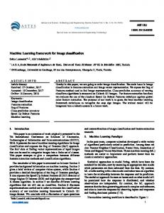
Fig. 1. Description of the Gray Level Co-occurrence Matrix.
Fig. 1. describes how to compute the GLCM. It shows an image and its corresponding co-occurrence matrix using the default pixels spatial relationship (offset = +1 in x direction). For the pair (2,1) (pixel 2 followed at its right by pixel 1), it is found 2 times in the image, then the GLCM image will have 2 as a value in the position corresponding to Ii =1 and Ij =2. The GLCM matrix is a 256x256 matrix; Ii and Ij are the intensity
D. Color GLCM GLCM has been defined for greyscale images. Extension to color images is straight forward. In color space the GLCM and its statistical features can be computed for each band. Comparisons can then be done between similar bands from two different images for classification. In this work, we computed the color GLCM in the following color spaces: RGB, HSL and La*b*. E. GLCM features distance GLCM features distance is obtained by computing the Euclidian distance between similar features for similar bands: 4
∆ GLCM =
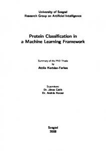
values for an 8bit image. The GLCM can be computed for the eight directions around the pixel of interest (Fig. 2.). Summing results from different directions lead to the isotropic GLCM and help achieve a rotation invariant GLCM. C. GLCM features From the GLCM we can compute different statistical measures. The following are used in this work: 1. Entropy: N −1
∑ − ln(P
i j ) Pi j
(1)
i, j =0
2.
Energy: Energy =
N −1
∑ (P
ij
i , j =0
)2
i
j
2
(6)
c =0
Fig. 2. Directions used for computing isotropic GLCM.
Entropy =
∑ (F [c] − F [c])
(2)
Where: F = [Entropy, Energy, Contrast, Homogeneity , Correlation] is the GLCM features vector (i for image 1 and j for image 2). F. Texture distance The global texture distance for each color band is computed by adding to the GLCM features distance, the square difference between entropies of the original band image: ∆ b = ∆ GLCM + ( Entrop i − Entrop j ) 2 (7) Where: Entrop i is the entropy of the original band image (i for image 1 and j for image 2). The final texture distance is the sum of the three color bands distances:
∆ Texture = ∆ b1 + ∆ b 2 + ∆ b 3
(8)
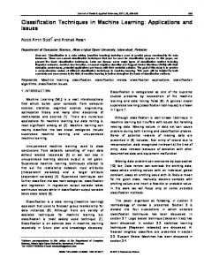
III. EXPERIMENTAL RESULTS For our experiments, we obtained a variety of industrial products from an industrial partner. These products are made of different materials: Fabric, wood, roofing shingles, leather, flooring vinyl materials, organic laminates, etc. 96 images were taken for building an image database. Tests were conducted on a subset of these images and some results are presented below. Examples of these images are given in Fig. 3. (Wood) and Fig. 4. (Roofing shingles).
W1
S1
S2
S3
S4
S5
S6
S7
S8
W2
W3
W4
W5
W6
W7
W8 S9
Fig. 3. Subset of wood images.
Fig. 4. Subset of roofing shingles images.
Our experimental setup is made of the following hardware and software: 1. A camera link 3-CCD high performance camera with a 1024x768 resolution and a 16mm F1.4 lens; 2. Fiber optic diffuse coaxial lighting with a 200W source;
3. 4. 5. 6.
Euresys Grablink Expert2 frame grabber; Intel Pentium P4 processor 2.0 GHz and 2GB Ram; eVision library for image acquisition; Matlab 7.3 (Release 2006B) and Image Processing Toolbox. The samples are placed at approximately 20cm from the
camera. The algorithms were implemented using Matlab 7.3, the Image Processing Toolbox and C++. The tests were conducted in RGB, HSL and La*b* color spaces. Table I and Table II give the obtained results for the images in Fig. 3. and Fig. 4. These results are for RGB color space which gives the best results in our experiments, followed closely by HSL color space. La*b* color space gives the worst results. The obtained results permit to effectively classify these images. TABLE I COLOR -TEXTURE DISTANCE IN RGB SPACE FOR WOOD IMAGES OF FIG. 3.
W1
W2
W3
W4
15,3
10,6 10,1
W2 W3
W5
W6
W7
W8
29,6
90,0
80,9
138,9
90,0
14,3
102,3
93,2
123,8
74,9
19,1
92,7
83,5
128,6
79,6
99,5
109,9
60,9
12,5
74,9
84,1
86,6
74,9
W4
108,7
W5 W6 W7
49,0
TABLE II COLOR -TEXTURE DISTANCE IN RGB SPACE FOR ROOFING SHINGLES IMAGES OF FIG. 4. S2 S1 S2 S3 S4 S5
1094
S3
S4
S5
S6
S7
S8
S9
with a variety of industrial samples and the obtained results are promising and show the possibility of efficiently classifying complex industrial products based on color and texture features. The color isotropic Gray Level Co-occurrence Matrix performed well in RGB and HSL color spaces. The La*b* color space does not permit to effectively discriminate between close color-texture samples. Classification between images was done successfully using a sum of color bands distances computed using isotropic GLCM. For each channel a sum of the Euclidian distance between GLCM features and the square difference between entropies of the original band images was used. Also of importance is the lighting used during the classification. We used a fiber optic coaxial diffuse lighting that permits a uniform diffuse lighting over the inspected surface. Other lighting techniques are planned for future tests. Future work includes: testing with other type of industrial samples, exploring the importance of different color bands in our texture analysis, exploring new ways of combining color and texture for classification, comparison with other texture classification techniques, and classification by means of neural networks. ACKNOWLEDGMENT Special thanks to M. Trudel, for providing product samples for our experiments and to CRVI technicians J. Poulin and L.A. Marceau (http://www.crvi.ca) who helped in building the image database.
97
163
250
1016
13
34
176
997
931
844
93
1081
1060
918
65
153
919
84
91
79
REFERENCES
87
853
149
129
13
R.C. Gonzalez , and R. E. Woods, Digital Image Processing 2nd Edition. Prentice Hall, 2002. [2] R.M. Haralick, K.Shanmugam, and I. Dinstein, “Textural Features for Image Classification”, IEEE Trans. on Systems, Man and Cybernetics, 1973, pp.610-621. [3] T. Caelli, and D. Reye, “On the classification of image regions by color, texture and shape”, Pattern Recognition, 26 (4), 1996, pp. 461-470. [4] M. Unser “Sum and Difference Histograms for Texture Classification”, IEEE Trans. on Pattern Analysis and Machine Intelligence, New York, 1986. [5] T. Ojala, and M Pietikainen, “Unsupervised texture segmentation using feature distributions”, Pattern Recognition 32 (3), 1999, pp. 477-486. [6] T. Ojala, M Pietikainen., and D. Harwood, “A comparative study of texture measures with classification based on feature distributions”, Pattern Recognition 29 (1), 1996, pp. 51-59. [7] L.J. Van Gool, P. Dewaele and A. Oosterlinck, “Texture analysis”, Computer Vision, Graphics, and Image Processing 29 (3), 1985, pp. 336-357. [8] A. Hanbury, U. Kandaswamy and D. A. Adjeroh, “Illumination-invariant Morphological Texture Classification”, 7th International Symposium on Mathematical Morphology, Paris, France 2005. [9] S. Majumdar, and D.S. Jayad, “Classification of cereal grains using machine vision: Combined morphology, color, and texture models”, Trans. of the American Society of Agricultural Engineers, vol. 43, 6, 2000, pp. 1689-1694. [10] M. Varma, and A. Zisserman, “Texture Classification: Are Filter Banks Necessary?”, IEEE Conference on Computer Vision and Pattern Recognition, 2003. [11] C.J. Setchell and N.W. Campbell, “Using Colour Gabor Texture Features for Scene Understanding”, 7th. International Conference on Image Processing and its Applications, 1999, pp. 372-376.
766
S6
237
216
74
1003
982
840
21
S7
163 142
S8
For wood, for example, we can see that for close images we have a good separation. The smallest distance is obtained between W2 and W3, followed by W1 and W3. These images are perceptually close and the obtained distances between these images give a good separation. The same conclusions are seen for roofing shingle images. For example, we can see that the smallest distances are obtained for perceptually close images (S1and S7, S4 and S9). These distances are large enough to permit a good separation between non-similar images. Tests conducted in other images in the database give similar interesting results. This is very promising for our framework and for the classification of complex color-texture industrial images. IV. CONCLUSION In this work we proposed a framework for a combined color and texture classification. The tests were performed
[1]
[12] D. Dennis, W.E. Higgins, and J. Wakeley, “Texture segmentation using 2D Gabor elementary functions”, IEEE Trans. on Pattern Analysis and Machine Intelligence, Vol. 16 (2), 1994, pp. 130-149. [13] J.H. Husoy, T. Randen, and T.O. Gulsrud, “Image texture classification with digital filter banks and transforms”, Proc. SPIE, Applications of Digital Image Processing XVI, Vol. 2028, 1993, pp. 260-271. [14] M. Mirmehdi and M. Petrou, “Segmentation of Color Textures”, IEEE Trans. on Pattern Analysis and Machine Intelligence, Vol. 22, 2, 2000, pp.142-159. [15] M. Pietikainen, T. Maenpaaand J. Viertola, “Color Texture Classification with Color Histograms and Local Binary Patterns”, Workshop on Texture Analysis in Machine Vision, 2002, pp.109-112. [16] M. Pietikainen, T. Maenpaaand J. Viertola, “Separating color and pattern information for color texture discrimination”, International Conference on Pattern Recognition, 2002, pp. 668-671. [17] A. Dimbarean, and P. Whelan, “Experiments in color texture analysis”, Pattern. Recognition Letters. Vol. 22, 2001. p.1161. [18] C.C. Chang, and L.L.Wang, “Color texture segmentation for clothing in a computer-aided fashion design system”, Image and Vision Compuing, 14 (9), 1996, pp. 685-702. [19] P. Chang and J. Krumm, “Object Recognition with Color Cooccurrence Histograms”, IEEE Conference on Computer Vision and Pattern Recognition, 1999, pp. 498-504. [20] K. Chen, and S. Chen, “Color texture segmentation using feature distributions”, Pattern Recognition Letters, 23, 7, 2002, pp. 755-771. [21] Y. Deng, and B.S.Manjunath, “Unsupervised segmentation of color-texture regions in images and video”, IEEE Trans. on Pattern Analysis and Machine Intelligence, 2001. [22] Y. Deng, B.S. Manjunath and H. Shin, “Color image segmentation”, IEEE Conference on Computer Vision and Pattern Recognition, 1999, pp.446-51. [23] Y. Deng and B.S. Manjunath, “An efficient low-dimensional color indexing scheme for region based image retrieval”, IEEE Internaional Conference on Acoustics, Speech and Signal Processing, 1999. [24] M. Hauta-Kasari, J. Parkkinen, T. Jääskeläinen,and R. Lenz, “Generalized cooccurrence matrix for multispectral texture analysis”, 13th International Conference on Pattern Recognition, 1996, pp. 785-789. [25] G. Van de Wouwer, P. Scheunders, S. Livens and D. Van Dyck, “Wavelet correlation signatures for color texture characterization”, Pattern Recognition, 32(3), 1999, pp. 443-451. [26] G. Van de Wouwer, B. Weyn and D. Van Dyck, “Multiscale, asymmetry signatures for texture analysis”, International Conference on Image Processing, 2004, pp. 1517-1520 [27] C.R. Dyer, T. Hong and A. Rosenfeld, “Texture classification using gray level cooccurrence based on edge maxima”, IEEE Trans. Systems, Man, and Cybernetics, 10, 1980, pp. 158-163. [28] A. Rosenfeld, W. Cheng-Ye, A. Wu, “Multispectral Texture”, IEEE Trans. on Systems, Man and Cybernetics, 1, 1982, pp. 79-84. [29] V. Arvis, C. Debain, M. Berducatand A. Benassi, “Generalization of the cooccurrence matrix for colour images : application to colour texture classification”, Journal of Image Analysis and Stereology, vol. 23, 2004, pp. 63-72. [30] S. Westland, and A. Ripamonti, Computational Colour Science. John Wiley, 2004. [31] A. Tremeau, C. Fernandez-Maloigne, and P. Bonton, Image numérique couleur. Dunod, 2004.