Support Vector Machine for Abnormal Pulse Classification - CiteSeerX

International Journal of Computer Applications (0975 – 8887) Volume 22– 22 No.7, May 2011

Support Vector Machin Machine for or Abnormal Pulse Classification Bhaskar Thakker

Anoop Lal Vyas

Indian Institute of Technology Delhi Instrument Design Development Centre Hauz Khas, New Delhi

Indian Institute of Technology Delhi Instrument Design Development Centre entre Hauz Khas, New Delhi

ABSTRACT Radial pulse signals have been utilized in ancient culture for the health diagnosis due to its simple,, non invasive and effective approach. Characteristics of a newly identified abnormal pulse in the subjects suffering from gastritis and arthritis are discussed along with commonly visible healthy pulse patterns in this work work. A binary classifier to segregate such abnormal pulse pulses from healthy pulse patterns is modeled using linear, quadratic as well as support vector machine ine based algorithms. Frequency domain features derived from power spectral density of the pulse signal are ranked to achieve dimensionality reduction. It has been found that the support vector machine with linear kernel classifies the abnormal pulse signals with highest success rate of 99.2% utilizing only two ranked frequency domain features.

General Terms Linear Classifier, Quadratic Classifier, Support Vector Machine, Kernel Function, Dimensionality Reduction

Keywords Radial pulse analysis, Distal pulsee point, Band Energy Ratio (BER), BAD Notch, Power spectral density

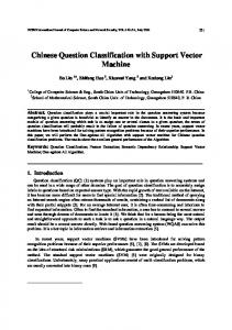
1. INTRODUCTION The radial pulse signal in human body has been utilized by modern medical science for examining the heart rate, systolic – diastolic blood pressure as well as arterial stiffne stiffness. These parameters are important for the subjects suffering from hypertension as well as atherosclerosis.. The radial pulse points have found to be practiced in ancient days in countries like China, India and Korea. The pulsations observed over three distinct inct pulse points were utilized for the assessment of not only the heart but also for the body organs like stomach, small and large intestine, bladder, kidney, liver, spleen and gall bladder. This traditional approach popular as Traditional Chinese Medicinee [1, 2] in China and as Ayurveda in India [3, 4], mention the use of three distinct pulse signals over a radial artery for thee health diagnosis as shown in Fi Fig. 1. The three pulse points are identified as Proximal (P), Middle (M) and Distal (D) pulse pointt with the reference to their location from heart. The characteristics of these six pulse signals of both the hands are reported in ancient literature summarizing all varities of diseases in human body. The pulse signals observed with finger tips are analyzed zed by the practitioner based on the nature of palpation identified over finger tip. The analysis is highly subjective and the prediction depends upon the experience and expertise gained by the practitioner.

Fig. 1: Traditional Approach of Radial Pulse Analysis A

The basic phenomenon behind establishment of pulse signal in the arterial structure is due to the ventricular ejection from heart which generates a forward wave in the arterial structure. The arterial channel consists of several branches and is finally f terminated in the form of several organs at the periphery. The forward pulse wave gets reflected from various peripheral organs like Kidney, Small Intestine, Large Intestine, Stomach etc., resulting into reflected waves in opposite direction. direction The combination mbination of forward wave and reflected wave establishes overall radial pulse morphology. The velocity with which the reflected wave travels is defined as pulse wave velocity. The pulse wave velocity and the nature of reflection from peripheral organ are the he key factors in establishing the overall pulse morphology in the arteries. The analysis of pulse morphologies in abnormal health conditions can prove to be of prime importance due to non invasive and simple approach of diagnosis followed here. Radial pulse pul analysis gives distinct importance to three pulse points identified as proximal, middle and distal pulse points for both the hands. The pulse signal observed over these three pulse points show several pulse patterns identified in literature as moderate, slippery, taut, wiry [5], suppressed dicrotic notch pulse and BAD notch pulse [9]. [ Time domain as well as frequency domain approaches are followed for feature extraction and pulse classifiers have been proposed by the researchers. The irregularities associated assoc with the pulse signal in cardiovascular problems have been identified with the help of sample entropy and such pulse is classified using support vector machine [55]. The pulse categories mentioned above have been classified using Daubichies wavelet of fourth order [6]. ]. Dynamic time warping algorithm has been utilized as a time domain approach for similarity measure of the pulse signal [7]. Fuzzy and Neural network based classifier has been applied on the feature vector prepared from several time domain pulse parameters like pulse height and width during systole and diastole phase, area under the pulse, pulse segment time etc. [8].

13

International Journal of Computer Applications (0975 – 8887) Volume 22– No.7, May 2011

Binary pulse classifier models segregating healthy pulse patterns and abnormal pulse patterns with BAD notch are presented here. Linear and quadratic classifiers are presented utilizing the frequency domain pulse features for this task. To further improve the generalization capability and classification accuracy, Support Vector Machine (SVM) has been used which classifies an abnormal pulse from commonly visible healthy pulse patterns with highest success rate.

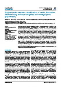
2. RADIAL PULSE ACQUISITION AND PREPROCESSING 2.1 Radial Pulse Characteristics The characteristics of a radial pulse signal is shown in Fig. 2. The radial pulse signal shows a rising wave due to systole phase of the heart when blood is pumped in the arterial channel though aorta. The systole phase ends when the aortic valve gets closed in the heart. Closing action of this aortic valve along with other peripheral factors results into formation of a dicrotic notch in the pulse signal [10]. The existence of reflected wave in the same arterial structure establishes average pulse wave. The falling pulse segment shows noticeable difference in healthy and unhealthy pulse patterns. The healthy pulse patterns usually show clear presence of dicrotic notch ‘DN’ as shown in Fig 1.

baseline fluctuations due to motion artifacts and respirations of the person giving frequency components in 0 to 0.5 Hz. This baseline fluctuations as well as static pressure component are removed using Daubichies wavelet transform ‘DB2’. The reconstructed signal from eighth level approximation coefficients of the pulse signal is subtracted to achieve dynamic pulse component.

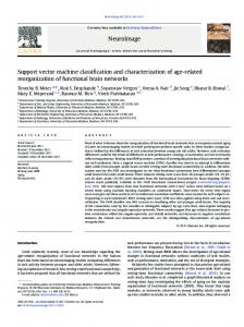
3. PULSE MORPHOLOGIES AND FEATURE EXTRACTION 3.1 Pulse Morphologies Pulse morphologies commonly visible in young and healthy subjects are shown in Fig. 3(a). The morphologies identified as Taut, Slippery or Moderate pulse according to Traditional Chinese Medicine clearly show the presence of dicrotic notch and dicrotic wave. An abnormal pulse pattern observed over the distal pulse point of either hand in the subjects suffering from gastritis or arthritis is shown in Fig. 3(b). The abnormal pulse pattern shows formation of a unique ‘V’ shaped notch identified as BAD Notch [9]. Out of 34 subjects 20 subjects suffering from chronic gastritis and 14 subjects suffering from arthritis have clearly shown the BAD notch formation in the end diastole phase of the pulse segment. The presence of such BAD notch is neither visible in the pulse signal corresponding to any other pulse point.

0.4 0.2 A(t)

According to the ancient Indian medicine formally known as Ayurveda, distal pulse point is believed to carry significant information about gaseous element in the human body. Gastritis and arthritis are the two disorders resulting from the vitiation or exaggeration of the gaseous element. The pulse signals acquired over the distal pulse point in the subjects of the above said disorders are examined. An abnormal pulse character visible in such subjects has been previously reported showing presence of a unique ‘V’ shaped notch, identified as BAD notch at the end of the pulse segment [9].

0

0.4 0.3

-0.2

A(t)

0.2

0

DN

0.1 0 -0.1

0.5

1 time (t)(sec)

1.5

(i) Taut Pulse

-0.2 0

0.2

0.4 time (t) (sec)

0.3

0.6

0.2

2.2 Radial Pulse Acquisition and Preprocessing A piezoresistive pressure sensor from Freescale Semiconductors having full scale range of 350 mmHg pressure is used for acquiring the radial pulse. The pulse signal is amplified using instrumentation amplifier and filtered to obtain a clean pressure signal. The signal is sampled at 500 Hz with the help of USB6009 Data Acquisition system from National Instruments. Since the radial pulse contains most of the signal in the lower frequency band, the signal is filtered with the help of a low pass filter having cut off frequency of 40 Hz. The signal also contains

A(t)

Fig. 2: Radial Pulse Signal Characteristics

0.1 0 -0.1 0

0.5 time (t) (sec)

1

(ii) Slippery Pulse

14


0.2

A(t)

0.1 0 -0.1 -0.2 0

0.5

1 time (t) (sec)

1.5

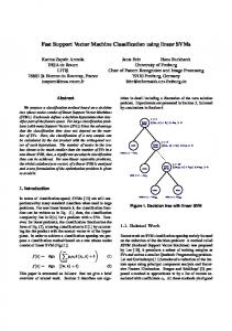
Welch's averaged modified periodogram method with Hamming window has been utilized for the power spectral density estimation. The periodogram for every pulse series having length in the range of 2000 to 2500 samples is derived with 1024 samples window length following 99% overlapping which gives 0.488 Hz frequency resolution. The distribution of the pulse energy in initial 0 to 20 Hz, are dependent on the rising slope and falling slope present in the pulse segment as well as overall pulse morphology. Power spectral density (PSD) for a healthy subject and an abnormal subject suffering from chronic gastritis has been shown in Fig. 4. The elevation of energy in frequency bands beyond 5 Hz is clearly visible in their power spectrums. Abnormal Subject Normal Subject

(iii) Moderate Pulse 0

Fig. 3: (a) Pulse Patterns in Healthy subjects Power/Frequency (dB/Hz)

0.15

A(t)

0.1 0.05 0

-10 -20 -30 -40 -50

-0.05 0

0.5 1 time (t)(sec)

1.5 BAD Notch

Fig. 3.: (b) Abnormal pulse pattern with BAD Notch

3.2 Pulse Feature Extraction The pulse signal shows significant information in the diastole phase to segregate normal and abnormal pulse patterns. Transformation of signal in frequency domain helps in representing the pulse features in terms of energies associated with individual frequency components. It is possible that the presence of BAD notch may elevate the energy associated with certain frequency components in the pulse spectrum. Hence power spectral density of the pulse is derived using Fourier transformation and then frequency bands of interest are investigated.

3.2.1 Features derived from power spectral density Power Spectral density of the signal has been defined as the magnitude squared of the Fourier transform of the real time signal of interest. Power spectral density from Discrete Fourier Transform of x (n) is achieved as

Where X ( k ) is the Discrete Fourier Transform (DFT) of a digitized signal x(n) and defined as

-60

0

5

10 Frequency (Hz)

15

20

Fig. 4: Power Spectral Density for Normal and Abnormal Subject To derive the frequency domain features from the PSD of pulse segment, the spectrum is divided in 1 Hz band. Since the energy beyond 20 Hz is found to be negligible in all the cases, only first 20 bands are retained. Energy in each band is divided by the total energy in 20 bands. The parameter Band Energy Ratio (BER) has then been defined as shown in eq. (3). For each pulse segment, BER values of 20 bands has been derived and used as a part of feature vector.

% !"! #$

3.3 Dimensionality Reduction The radial pulse signal is established due to pumping action in the heart. The heart rate is usually in the range of 60 beats per minute to 130 beats per minute. Hence the pulse pressure signal is a low frequency signal. But in abnormal health conditions the nature of the peripheral reflected signal could give rise to larger amount of harmonics of the fundamental frequency component. Hence the frequency components in the range of 0.5 Hz to 20 Hz have been accepted for preparing feature vector. From classification point of view, there may be redundancies existing among these frequency components. The dimensionality of the feature vector can be reduced by either identifying the correlated features or identifying the features that have great influence in classification task. To follow the second approach, it is desired

15

International Journal of Computer Applications (0975 – 8887) Volume 22– No.7, May 2011 to retain only those frequency components which are significant for classification task. The frequency components should be ranked according to their classification power and group of only these frequency components should be used for classification purpose. This approach not only provides dimensionality reduction for the feature vector but also adds on the performance part of the classifier. For each of the Band Energy Ratio (BER) of 1 Hz band, in the range of 0.5 Hz to 20 Hz, a histogram as shown in Fig. 5 is prepared for both the groups under study. Based on two sample t-test with pooled variance estimate, the statistical difference between BERs is estimated. The greater difference in means of two BERs helps in achieving better classification accuracy. The BERs are ranked based on this statistical difference. Table 1 shows initial 10 ranked BERs derived according to their classification power.

A Linear Discriminant function is defined as:

& ' & (

where coefficients ‘wi ’ are the components of weight vector ‘w’ and ‘x’ is a d-dimensional feature vector derived from the ranked frequency components of the pulse signal. Linear Discriminant classifier requires )1+d*Mcoefficients for ddimensional feature vector and M class problem. Another classifier using Quadratic Discriminant function utilizes additional term for the product of pairs of feature vector elements of ‘x’. A Quadratic Discriminant function is defined as:

8 Normal Subject Abnormal Subject

7

4.1 Linear and Quadratic Pulse Classifier Design

Number of Subjects

6

& ' & ' & +

5

4

Using Quadratic Discriminant classifier, with d dimensional feature vector for M class problem, number of weights required

3

'

will be)'' *,.. Since quadratic classifier uses the product of features term, it helps in defining non-linear decision boundary. In both of these classifiers distinct value of g(x) is chosen for each class and weight vector ‘w’ is trained with the help of pulse feature vector ‘x’ [11].

2 1 0

0

0.05 0.1 Band Energy Ratio for a Frequency Band

0.15

Fig. 5: Histogram of both the groups for ith freuqency component

Table 1. Ranking of the Band Energy Ratios Ranked Parameter 1 2 Frequency 19 16 Band

3

Rank of the Band 4 5 6 7

8

9

10

17

11

13

12

10

18

20

14

4. PULSE CLASSIFIER DESIGN The classification is a task of function approximation where a function that maps a d-dimensional input to a correct class label is desired. The feature space is linearly separable then in that case a simple linear function can be derived in the form of a decision boundary. Hence a linear classifier must be tried as a first attempt. Most of the real life problems are having some overlapping regions in the feature space due to noise present in the data as well as limited availability of the data. Hence a nonlinear approximation function is desired in such case to define a decision boundary that can provided better classification accuracy. A comparison of several classifier models including (i) Linear discriminant function, (ii) Quadratic discriminant function and (iii) Support Vector Machine has been carried out.

4.2 Pulse Classifier using Support Vector Machine Support Vector Machine (SVM) belongs to a family of generalized linear classifiers which is based on maximization of the margin between two sets of data [12]. SVM as a supervised learning algorithm is popular for classification and regression task due to its ability to generalize well for unknown data set avoiding over-fitting of the data. SVM has been successfully applied for the classification task in biomedical signals like ECG and EEG, DNA pattern as well as face recognition [13 - 15]. Many biological problems involve high-dimensional, noisy data, for which SVMs have proven better compared to any other statistical or machine learning methods. The basics of SVM algorithm is briefly mentioned here details for which can be found in [16]. The margin of a linear classifier in SVM is defined as the distance from the closest training sample to the decision boundary. SVM is binary classifier and the discriminant function value g(x) holds ± 1 for two classes. The margin is as 1.-w- where -w- is the norm of w. In non linear separable case it is difficult to find hard margin with zero classification error. Hence a slack variable /0 is introduced to allow misclassification for few training data samples near the marginal hyperplane. The optimization problem in search of decision boundary results into following equation.

16


1 -&- '3 / &2

456!7 8&2 9':/ 2/ :;!22

The training samples for which =0 9 are called support vectors and only these training samples are enough for determining the weight vectors. The coefficients=0 are found by maximizing the following quadratic programming problem.

2

?= = = = @ A

B56!7C= C322D =

The decision function can be achieved from =0 using support vectors 'nsv ' as nsv

fx = sign E yi αi .x.xi + bF

(9)

i=1

where signum function 4 G

'9H "4

A non linear kernel function can be applied on the feature vector to transform it in the higher dimensional space which helps SVM to find a linear boundary. Here the task is achieved at the cost of increased complexity of the classifier due to increase in dimensions. The kernel trick [14] allows computationally efficient way of maintaining the same dimension in original feature space along with achieving linear separation among groups. The feature vectors which are having non linear boundary in original feature space can result in to a linear separable case once transformed into higher dimensional kernel space. A non linear kernel function having the form shown in eqn. (10) can be helpful in working with the transformed kernel space without increasing dimension along with utilizing its non linear features in classifying the problem with linear decision boundary. In absence of this kernel trick the complexity increases quadratically.

The polynomial kernel with degree d defined as I 2 J @ ' is following to eqn. (10) and Mercers conditions to qualify for utilizing Linear SVM. The decision boundary after the application of kernel function becomes

; 4 E = @Г @ 'F

The choice of kernel function is data dependant and usually linear kernel is tried as first attempt due to its less convergence time as well as small number of parameters required to train the classifier. Hence SVM with polynomial kernels with degree 1 to 4 have been applied on the pulse database.

4.3 Performance Evaluation of the classifier The Band Energy Ratios (BERs) after ranking are used as the feature vector. It is required to identify the requirement of number of initial ranked features to achieve highest accuracy for the problem under study. It is often found that when number of features exceed beyond certain stage, the accuracy of the classifier degrades for the unknown data. This is due to the fact that during training procedure; the classifier achieves a very specific solution when trained with large amount of features. Such a trained classifier lacks of generalization capability. Hence the classifier is required to be trained with sequential group of initial ranked features and test accuracy is required to be derived for each of the group. Final classifier model with certain number of input features will be selected based on the highest achievable accuracy for the unknown data set. A pulse database containing the pulse recording of 22 abnormal subjects with chronic gastritis and arthritis and 31 young healthy subjects has been defined. Band Energy Ratio for 0 to 20 Hz has been carried out after deriving power spectral density of the subjects. The BERs are ranked and ordered to form a feature vector. The pulse data set is divided into training and test data set using 5 fold cross validation. Linear, quadratic as well as SVM classifier with polynomial kernel 1, 2, 3 and 4 are trained. In each of the iteration of 5 fold cross validation, the classifier is trained 25 times and then results are averaged for that iteration. After having trained, the classifier is tested with unknown test data set. The parameters that can help in examining the performance of a classifier are as following. B4MB BO6P6B Q6656Q

'N

'N

'

%

' 'N 'N

(

where, TP is True Positive, TN is True Negative, FP is False Positive and FR is False Negative. Sensitivity is the fraction of subjects with the disease that the test correctly classifies as positive. On the other hand specificity is the fraction of subjects without disease that the test correctly classifies as negative. I 2 JK @K Accuracy gives the total subjects correctly classified out of all the subjects under consideration.

17


5. RESULTS AND DISCUSSION The test accuracy for linear as well as quadratic classifiers is shown in Fig. 6. The highest achievable accuracy with linear classifier is 91% for initial 5 ranked features. On the other hand quadratic classifier improves on accuracy as 94% for just 2 initial ranked features. In these classifiers the approximation function derived as a part of training is not the optimum one. The training procedure is stopped when the criteria of mean squared error is reached. Hence out of so many possible approximation functions in the feature space, the one that is optimum is not available with these classifiers. Table 2 shows the sensitivity and specificity for these classifiers along with their accuracies.

Table 2. Linear and quadratic classifier performance Classifier Linear Quadratic

A (%) 91.0 94.0

SN (%) 78.23 95.18

SP (%) 100 93.15

Number of features 5 2

Linear Classifier Quadratic Classifier 95

% Test Accuracy

90

calculations of α i that defines the weight vector of decision boundary resulting into under fit of the data, which is also not desired. So, the optimum value of C is chosen based on the performance of the classifier for the unknown test data set. It is desired to have an SVM model with higher classification parameters along with maximum margin, less complexity in terms of lower value of C and small number of support vectors. The performance of the SVM classifier model with polynomial kernel having degrees from 1 to 4 is shown in Table 3. SVM trained with linear kernel (polynomial order = 1) gives highest test accuracy as 99.2% with 100% sensitivity and 98.2% specificity with 19 support vectors among all the four classifiers. The optimum value of the soft margin constant C to achieve this highest accuracy is found to be 100 for linear kernel SVM. Figure 7 shows the classification accuracy for sever group of initial ranked features for linear kernel SVM and Fig. 8 shows the decision boundary derived using support vectors.

Table 3. Polynomial Kernel SVM Classifier performance with initial 2 ranked features Polynomial Kernel degree 1 2 3 4

A (%)

SN (%)

SP (%)

99.2 98.4 98.0 98.8

100 100 100 99.16

98.2 96.4 94.66 98.12

Number of Soft Support Margin Constant Vectors 19 100 26 10 36 0.1 31 1

85 C = 0.1 C=1 C = 10 C = 100 C = 1000 C = 10000

80

75

100

5 10 15 Group of Ranked Frequency Domain Features

Fig. 6: Classification accuracy with linear and quadratic classifiers A classifier based on Support Vector Machine is used for the database because SVM tries to find an optimum hyperplane out of all possible hyperplanes in the transformed kernel space. Hence the result available with SVM is having better generalization capability. In case of SVM, the performance of the classifier model depends of the parameters like kernel function being used and soft margin constant C. The value of C decides the margin between the upper and lower marginal hyper planes. Higher value of C results in to reduction in the margin and infinite value of C is a case of Hard margin SVM. SVM introduces large amount of penalty on the training errors for higher values of C. In such situations, SVM tries to find a perfect separation between two groups resulting into overfitting which is not desired. On the other hand when C is kept very small, less penalty is introduced on training errors and the margin increases. Here SVM puts high constraints on

% Test Accuracy

95 90 85 80 75 70 0

5 10 15 Group of Ranked Features

20

Fig. 7: Classification Accuracy for Linear kernel SVM

18

International Journal of Computer Applications (0975 – 8887) Volume 22– No.7, May 2011 0.22 0 1 Support Vectors

0.2 0.18

Ranked Feature 2

0.16

[5] Jianjun Yan, Yiqin Wang, Fufeng Li, Haixia Yan, Chunming Xia, Rui Guo “Analysis and Classification of Wrist Pulse using Sample Entropy”, Proceedings of IEEE International Symposium on IT in Medicine and Education, 2008 pp. 609 – 612. [6] L S Xu, K Q Wang, L Wang, “Pulse waveforms Classification Based on Wavelet Network” Proceeding of IEEE Engineering in Medicine and Biology 27th Annual Conference, Shanghai, china, 2005 pp. 4596-4599.

0.14 0.12 0.1 0.08

[7] L U Wang, Kuan-Quan Wang, Li-Wheng Xu “Recognizing Wrist Pulse Waveforms with Improved Dynamic Time Warping Algorithm” Proceedings of the Third International Conference on Machine Learning and Cybernetics, Shanghai, 2004; pp. 3644 -3699.

0.06 0.04 0.02 0

0.02

0.04 0.06 Ranked Feature 1

0.08

Fig. 8: Identification of decision boundary using support vectors

6. CONCLUSION An abnormal pulse pattern identified with the presence of BAD notch in the subjects of chronic gastritis and arthritis is classified using linear, quadratic as well as support vector machine algorithms. SVM proves to be better than any other algorithm due to its capabilities to generalize well by searching a decision boundary with maximum margin. The features derived from power spectral density of the pulse series are ranked to achieve dimensionality reduction. Only two ranked features that is Band Energy Ratio (BER) for 19th and 16th band are sufficient to classify the BAD Notch pulse with highest classification accuracy of 99.2% using linear kernel SVM.

7. ACKNOWLEDGMENTS We are thankful to New Delhi Municipal Council (NDMC), India for providing facilities for acquiring wrist pulse signals. Partial support from a collaborative project under the UK India Education Research Initiatives (UKIERI) is also thankfully acknowledged.

8. REFERENCES [1] B. Flaws “The Secrets of Chinese Pulse Diagnosis”, 1995 Blue Poppy Press, Boulder, CO. [2] Wang, Shu-ho., “The Pulse Classic”, 1997 Blue Poppy Press, Boulder, CO. [3] V. Dattatray Lad “Secrets of the Pulse the Ancient Art of Ayurvedic Pulse Diagnosis” Motilal Banarasidas Publishers INDIA, 2005.

[8] L S Xu, Max Q H Meng, K Q Wang “Pulse Image Recognition Using Fuzzy Neural Network” Proceedings of the 29th Annual International Conference of the IEEE Engineering in Medicine and Biology, France, 2007; pp.3148 - 3151. [9] Bhaskar Thakker, Anoop Lal Vyas “Radial Pulse Analysis at Deep Pressure in Abnormal Health Conditions” Third International Conference on BioMedical Engineering and Informatics, October, 2010; pp. 1007-1010. [10] Gordon A. Ewy, Jorge C. Rios and Frank I. Marcus “The Dicrotic Arterial Pulse” Circulation: Journal of American Heart Association, Vol. 39, May 1969, pp. 655 – 661. [11] Richard O. Duda, Peter E. Hart, David G. Stork Pattern Classification. Second edition Wiley, 2006. [12] C. Cortes and V. Vapnik, “Support-vector networks,” Machine Learning, vol. 20, no. 3, pp. 273–297, 1995. [13] Asa Ben-Hur, Cheng Soon Ong, Soren Sonnenburg, Bernhard Scholkopf and Gunnar Ratsch, “Support Vector Machines and Kernels for Computational Biology” PLOS Computational Biology Vol. 4, October 2008. [14] D. Alvarez-Estevez, V. Moret-Bonillo, “Identification of Electroencephalographic Arousals in Multichannel Sleep Recordings”, IEEE Transactions on Biomedical Engineering, Vol. 58, No. 1, January 2011, pp. 54 – 63. [15] B. E. Boser, I. M. Guyon, and V. N. Vapnik, “A training algorithm for optimal margin classifiers,” in Proc. 5th Annu. ACM Workshop Computational Learning Theory (COLT), Pittsburgh, PA, 1992, pp. 144–152. [16] V. N. Vapnik, Statistical Learning Theory. New York: Wiley, 1998.

[4] S. Upadhyaya “Nadi Vijyaya Ancient Pulse Science” Chaukhamba Publishers, INDIA 2005.

19