Support Feature Machine for Classification of Abnormal ... - CiteSeerX

Research Track Paper

Support Feature Machine for Classification of Abnormal Brain Activity ∗

W. Art Chaovalitwongse and Ya-Ju Fan

Rajesh C. Sachdeo

Dept. of Industrial and Systems Engineering Rutgers University Piscataway, New Jersey, USA

Dept. of Pediatrics Jersey Shore University Medical Center Neptune, New Jersey, USA

[email protected], [email protected]

[email protected]

ABSTRACT

1.

In this study, a novel multidimensional time series classification technique, namely support feature machine (SFM), is proposed. SFM is inspired by the optimization model of support vector machine and the nearest neighbor rule to incorporate both spatial and temporal of the multi-dimensional time series data. This paper also describes an application of SFM for detecting abnormal brain activity. Epilepsy is a case in point in this study. In epilepsy studies, electroencephalograms (EEGs), acquired in multidimensional time series format, have been traditionally used as a gold-standard tool for capturing the electrical changes in the brain. From multi-dimensional EEG time series data, SFM was used to identify seizure pre-cursors and detect seizure susceptibility (pre-seizure) periods. The empirical results showed that SFM achieved over 80% correct classification of per-seizure EEG on average in 10 patients using 5-fold cross validation. The proposed optimization model of SFM is very compact and scalable, and can be implemented as an online algorithm. The outcome of this study suggests that it is possible to construct a computerized algorithm used to detect seizure pre-cursors and warn of impending seizures through EEG classification.

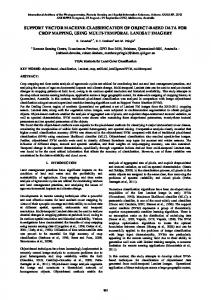
The human brain is among the most complex systems known to man. The rapidly growing technology in the past decade has made it possible for physicians to capture simultaneous responses from brain functions to test many longstanding brain theories. Almost all experiments in brain research have resulted in massive amounts of data. Often time, the captured information flood from brain diagnosis like neuroimaging and neurophysiological signals is in the form of large spatial and temporal data, also known as multidimensional time series (MDTS). Very few studies in brain research and data mining have been tailored to exploit both spatial and temporal properties of these brain data [4, 28, 32]. The exploration of such massive medical data requires very efficient and sophisticated techniques capable of capturing both spatial and temporal properties simultaneously. In this research, we herein propose a novel spatio-temporal classification technique, called support feature machine (SFM), used to classify multi-dimensional time series data. Epilepsy is a case in point in this study. An application of SFM will be demonstrated through the classification of normal and abnormal (pre-seizure) brain activity using electroencephalograms (EEGs) data. EEG, acquired in MDTS format, has been traditionally used as a tool for capturing the electrical changes and evaluating physiological states (normal and abnormal) of the brain. SFM can be used in developing a novel online classification paradigm that can accurately and reliably differentiate pre-seizure from normal EEGs. As seizure occurrence is always believed to be random, the classification framework proposed in this study is among the pioneering attempts to tackle the seizure prediction challenge [16, 19]. The outcome of this study may improve the medical diagnosis and prognosis in epilepsy as well as other abnormal brain functions like sleep disorders, movement disorders, and cognitive disorders. In addition, SFM can also be applied to other real life spatio-temporal data mining problems like anomaly detection or event prediction problems. A typical electrode montage for intracranial EEG recordings used in our study is shown in Figure 1a, which is a modified image of brain anatomy in [26]. An emerging view in recent epilepsy research suggests that there are four stages evolved in the seizure process: normal, pre-seizure, seizure onset, and postseizure [16, 19]. The state transition of seizure evolution has also been confirmed by our previous studies [6, 5, 29] and other groups [24, 14, 9]. The 10-second EEG profiles during these stages are illustrated in Figures 1b.

Categories and Subject Descriptors I.5.4 [Pattern Recognition]: Applications—signal processing, waveform analysis

General Terms Algorithms, Design, Experimentation, Performance

Keywords classification, time series, epilepsy, optimization ∗ This material is based upon work supported by the National Science Foundation under Grant No. 0546574.

Permission to make digital or hard copies of all or part of this work for personal or classroom use is granted without fee provided that copies are not made or distributed for profit or commercial advantage and that copies bear this notice and the full citation on the first page. To copy otherwise, to republish, to post on servers or to redistribute to lists, requires prior specific permission and/or a fee. KDD’07, August 12–15, 2007, San Jose, California,USA. Copyright 2007 ACM 978-1-59593-609-7/07/0008 ...$5.00.

113

INTRODUCTION

Research Track Paper

ROF RST

43 21

1234

4321 1 2 3 4 5

1 2 34 1 2 3 4 5

RTD

LOF LST

LTD

(a)

1

2

3

4

(b)

Figure 1: (a) Inferior transverse views of the brain, illustrating approximate depth and subdural electrode placement for EEG recordings, are depicted. Subdural electrode strips are placed over the left orbitofrontal (LOF), right orbitofrontal (ROF), left subtemporal (LST), and right subtemporal (RST) cortex. Depth electrodes are placed in the left temporal depth (LTD) and right temporal depth (RTD) to record hippocampal activity; (b) Twenty-second EEG recordings of (b1) Normal Activity (b2) Pre-Seizure Activity (b3) Seizure Onset Activity (b4) Post-Seizure Activity from patient 1 obtained from 32 electrodes. Each horizontal trace represents the voltage recorded from electrode sites listed in the left column (see for anatomical location of electrodes).

1.1

Epilepsy and Abnormal Brain Activity

Bayesian models) and optimization (e.g., neural networks) for classification techniques. Since this paper is focused on a new optimization model for MDTS data, we give a short review on previous studies using optimization for classification. Generally, classification techniques are combinatorial in nature as they involve discrete decisions (assignment of data points into a class). Thus, classification problems can be naturally posted as discrete optimization problems [10, 20]. The research in developing discrete optimization for classification problems is not new. The pioneering work was introduced in the 60’s [20]. Nevertheless, optimization in classification and data mining research is still very challenging and remains intractable because the goal classification naturally lends itself to a discrete optimization problem. Aside from the complexity issue, the massive scale of real life classification problems is another difficulty arising in optimization in data mining research. There have been enormous number of optimization techniques for classification problems developed during the past few decades including classification tree, support vector machines (SVMs), linear discriminant analysis, logistic regression, least squares, nearest neighbors, etc. For example, there are a number of linear programming formulations for SVMs proposed to explore the properties of the structure of the optimization problem and solve large-scale problems [2, 21]. There have been a few studies in data mining investigating the application of data mining techniques in MDTS classification problems. Guyon et al. (2002) [13] proposed a new feature subset selection (FSS) technique, recursive feature elimination method, to pre-process MDTS data or multivariate time series, before using SVM to classify cancer genes. Subsequently, Yang et al. (2005) [36] proposed an improved FSS technique that utilizes the correlation coefficient matrix.

Epilepsy can be broadly defined as recurring seizures – sudden, brief changes in the way the brain works [8]. The most disabling aspect of epilepsy is the uncertainty of recurrent seizures, which can be characterized by a chronic medical condition produced by temporary changes in the electrical function of the brain. Although neurological signals like EEGs offer good spatial and excellent temporal resolution to characterize rapidly changing electrical activity of brain activation, neuroscientists understand very little about the dynamical transitions to neurological dysfunctions of seizures. The unpredictable occurrence of seizures has presented special difficulties regarding the ability to investigate the factors by which the initiation of seizures occurs in humans and how to prevent seizures from happening. If seizures could be anticipated, it would lead to the development of completely novel diagnostic and therapeutic advances in controlling epileptic seizures. Finding hidden patterns or relationships in EEG data may offer a possibility to better understand brain functions from a system perspective, which will generally be very useful in medical diagnosis. Thus, the necessary first step to advance research in seizure prediction is to develop novel techniques capable of recognizing and capturing epileptic activity in EEGs before seizures occur. The discriminant ability to detect the seizure susceptibility period (seizure precursor) is logically a prerequisite of seizure prediction/warning development.

1.2

Optimization and Classification

Classification has been used for a wide variety of tasks in data mining. There are a wide variety and technical sophistication of the classification techniques. For example, there is a rich body of work in both statistical modeling (e.g.,

114

Research Track Paper

1.3

Contribution of the Paper

2.1

This paper proposes a novel spatio-temporal classification technique to enhance the ability to classify MDTS data. The proposed technique can be used to discriminate preseizure EEG signals (seizure pre-cursor) from normal EEG signals. One of the most challenging aspects in this study is the fact that EEG data are massive with an average over 300,000 data points per 1-minute of all electrode recordings. We propose an EEG feature extraction technique based on the chaos theory to reduce the dimensionality of EEG data. Since MDTS data like EEGs have properties in space and time, good MDTS classification techniques should be able to incorporate both spatial and temporal characteristics. To the best of our knowledge, this study represents the first attempt to formulate an optimization model to capture spatiotemporal properties for MDTS classification. The proposed technique, SFM, can incorporate both spatial and temporal properties by employing statistical time series analysis and the nearest neighbor rule within the optimization model. The SFM optimization model is to select the dimensions (features) of the MDTS that will maximize the correct classification subject to the nearest neighbor rule on inter-class and intra-class time series statistical distances. The optimal features that maximize the classification accuracy will be selected and used in the testing phase. The solution to an SFM problem is also easy for the end users (e.g., physicians) to interpret. For instance, in our case, the SFM solution is a group of electrodes that show the most discriminating power in normal and pre-seizure EEG classification.

1.4

Quantification of the brain dynamics from EEGs in this study is suitable to the extraction of EEG data because it is capable of automatically identifying and appropriately weighing existing transients in the EEG data. This technique is motivated by mathematical models from chaos theory used to characterize multi-dimensional complex systems and reduce the dimensionality of EEGs [25, 33]. To quantify the brain dynamics, we divide EEG signals into sequential 10.24-second epochs (non-overlapping windows). To properly account for possible nonstationarities in EEG signals, we chose the window size of 10.24-second (or 2048 EEG data points) such that it is large enough to capture the periodic motion and small enough to satisfy the stationarity assumption [22]. For each epoch of each channel of EEG signals, we estimate the measure of chaos, known as Short-Term Maximum Lyapunov Exponent (ST Lmax ), to quantify the chaoticity of the attractor using the method proposed in [17, 15]. A chaotic system like human brain is a system in which orbits that originate from similar initial conditions or nearby points in the phase space diverge exponentially in expansion process. The rate of divergence is an important aspect of the dynamical system and is reflected in the value of Lyapunov exponents. In other words, the Lyapunov exponents measure the average uncertainty along the local eigenvectors of an attractor in the phase space [34]. Next, we will give a short overview of mathematical models used in the estimation of ST Lmax from EEG signals.

2.1.1

Paper Organization

EEG Time Series Embedding

The initial step in extract dynamical features from EEG signals is to embed data from each EEG channel in a higher dimensional space of dimension p. This technique is known as the method of delays [33], which is used to capture the temporal behavior of the p variables that are primarily responsible for the dynamics of the EEG. We can construct p-dimensional vectors X(t), whose components consist of values of the recorded EEG signal x(t) at p points in time separated by a time delay as:

The organization of the succeeding sections of this paper is as follows. In Section 2, the method used to extract features from EEG data, statistical measures in time series analysis, and optimization models for SFM are described. The EEG data description and experimental design are presented in Section 3. The classification results and the performance characteristics of the proposed technique are addressed in Section 4. The concluding remarks are given in Section 5.

2.

EEG Feature Extraction

Xi = (x(ti ), x(ti + τ ) . . . x(ti + (p − 1) ∗ τ ))

METHODOLOGY

(1)

where τ is the selected time lag between the components of each vector in the phase space, p is the dimension of the embedding phase space, and ti ∈ [1, T − (p − 1)τ ]. In this study, we use p = 7 and τ = 3 as it was shown to be the most appropriate setting (i.e., best trade-off between the computational effort and epileptic activity characterization) [15]. An EEG signal embedded in the phase space are illustrated in Figure 2.

The spatio-temporal classification framework developed in this study is comprised of 3 key steps. The first step is the feature extraction from multi-channel EEG data. In this study, we employ a quantitative measure of brain dynamics from EEG data. The measure of brain dynamics, based on the chaos theory, has been previously shown capable of contemplating dynamical mechanisms of the brain network from EEG signals [15]. After the brain dynamical measure for each EEG channel is calculated, the subsequent step is the selection of time series similarity measures. We herein employ 3 time series similarity measures to the analysis of brain dynamics in EEG time series. Those measures include Euclidean, T-Statistical, and Dynamic Time Warping distances. The third step is the classification algorithm, which is based on optimization models used to classify unlabeled samples based on the nearest neighbor rule. Integration of the optimization models and the nearest neighbor rule results into a novel MDTS classification technique, called SFM, which is used to classify normal and pre-seizure EEGs in this study.

2.1.2

Estimation of Short-Term Maximum Lyapunov Exponent (ST Lmax )

The method for estimation of ST Lmax for nonstationary data (e.g., EEG time series) is previously explained in [15, 34]. In this section, we will only give a short description and basic notation of our mathematical models used to estimate ST Lmax . Define Na as the number of local ST Lmax ’s that will be estimated within a duration T data segment. If we define Dt as the the sampling period of the time domain data, we then have T = (N − 1)Dt = Na ∆t + (p − 1)τ . Let X(ti ) be the point of the fiducial trajectory φt (X(t0 )) with t = ti , X(t0 ) = (x(t0 ), . . . , x(t0 + (p − 1) ∗ τ )), and X(tj ) be a properly chosen vector adjacent to X(ti ) in the phase

115

Research Track Paper

Figure 2: Diagram illustrating an EEG epoch embedded in phase space for the quantification of brain dynamics: assume p = 4. The fiducial trajectory, the first three local Lyapunov exponents (L1 , L2 , L3 ), is shown. space. Define δXi,j (0) = X(ti ) − X(tj ) as the displacement vector at ti , i.e., a perturbation of the fiducial orbit at ti , and δXi,j (∆t) = X(ti + ∆t) − X(tj + ∆t) as the evolution of this perturbation after time ∆t. Denote ti = t0 + (i − 1) ∗ ∆t and tj = t0 + (j − 1) ∗ ∆t, where i ∈ [1, Na ] and j ∈ [1, N ] with j 6= i. Let ∆t be the evolution time for δXi,j , i.e., the time one allows δXi,j to evolve in the phase space. t0 is defined as the initial time point of the fiducial trajectory and coincides with the time point of the first data in the data segment of analysis. In the estimation of ST Lmax , for a complete scan of the attractor, t0 should move within [0, ∆t]. Finally, ST Lmax is defined as the average of local Lyapunov exponents in the state space and can be calculated by the following equation: ST Lmax =

2.2

Na |δXi,j (∆t)| 1 X log2 . Na ∆t i=1 |δXi,j (0)|

(2)

Constructing Distance Matrix: Similarity Measures

In this study, the choice of similarity measures is a very important step in achieving accurate classification results. To our knowledge, we are the first to develop a framework incorporating statistical time series similarity measures for differentiating EEG signals from normal and pre-seizure states. We will also apply and compare the performance of those similarity measures, including Euclidean, T-Statistical (index), and Dynamic Time Warping distances. Each of these measures can give us different aspects and insights about temporal and spatial characteristics of EEG signals.

2.2.1

alignment matrix will then be constructed by using the Euclidean distance as the local distance between two vectors, d(xi , yj ) = (xi −yj )2 , where the (ith , j th ) element of the matrix is the distance d(xi , yj ) between the ith point of time series X, and the j th point of time series Y . Subsequently, we construct a warp path, W = w1 , . . . , wK , starting at the beginning of each time series, w1 = (1, 1), and finishing at the end of both time series, wK = (n, n). Note that K is the length of the warp path and max(|X|, |Y |) ≤ K < |X| + |Y |. The kth element of the warp path represents the matching point of two time series, wk = (i, j), where (i, j) corresponds to index i from time series X, and index j from time series Y (shown in Figure 3). There is also another constraint on the warp path to be monotonically increasing in indices. Specifically, if wk = (i, j) and wk+1 = (i0 , j 0 ), then a warp path must satisfy i ≤ i0 ≤ i + 1 and j ≤ j 0 ≤ j + 1. There exist an exponential number of warping paths that satisfy the above conditions. However, the optimal warp path is the one with a minimum warping (distortion) cost defined K P 1 d(wki , wkj ). Using a dynamic by Dalign (X, Y ) = min K k=1

programming approach, the warp path must either be incremented by one unit (adjacent) or stay at the same i or j axes. Therefore, we only need to evaluate the recurrence of the cumulative distance found in the adjacent elements: 8 < D(i, j − 1) D(i − 1, j) D(i, j) = d(xi , yj ) + min : D(i − 1, j − 1). This results into the optimality condition for the warping ∗ ∗ path: DT Wxy (wk ) = d(xi(k) , yj(k) , wk )r(wk )+DT Wxy (wk−1 ). In this study, we employ an additional global constraint on the warping path described in [27, 35]. The main idea of this additional constraint is to speed up DTW distance calculation as well as to prevent pathological warping. Pathological warping occurs when a relatively small section of one sequence maps onto a relatively large section of another. The global constraints, known as Sakoe-Chiba band [30], is given by Y − r ≤ X ≤ Y + r, where r = 3, 5, 7, 9 (see Figure 3 when r = 3). Here, we treat r as a parameter in our DTW distance calculation and we will pick the best value of r empirically (i.e., the value that yields the maximum classification accuracy).

Dynamic Time Warping (DTW) Distance

Give two time series (or vector sequences) X and Y of equal length |X| = |Y | = n, DTW is a distance (similarity) measure used to compute the best alignment warp between time series X and time series Y with the minimum distortion. DTW has been widely used in many contexts including data mining [18, 1], gesture recognition [12], speech processing [31], and medicine [3]. The DTW distance can be calculated by using a dynamic programming approach. First, construct an alignment of every data point in time series X to match with every point in time series Y . The n×n

116

Figure 3: Warping Paths and Global Constraints: A warping matrix and a constrained warping matrix with the minimum-distance warp path of two time series X and Y .

Research Track Paper

2.2.2

Feature 1

T-Statistical Distance (T-index)

The t-test is commonly used to determine if two time series differ from each other in a significant way under the assumptions that the paired differences are independent and identically normally distributed. Note that the t-test deals with the problems associated with inference based on small samples (epochs of time series), which implies that the calculated mean and standard deviation may deviate from the “real” mean and standard deviation. The t-index is a similarity degree from the paired t-test for comparisons of means of paired-dependent observations. In this study, we use the t-index as a measure of statistical distance between two time series. Specifically, it is used to estimate the difference of the EEG signals from different brain states. The t-index, Txy , between the time series X = x1 , . . . , xn and Y = y1 , . . . , yn n P

i=1

Normal

Feature 2

A Feature 3

Figure 4: The nearest neighbor query starts at the test point and grows a spherical region until it encloses k training samples, and it labels the test point by a majority voting of these samples.

|xi −yi |

variables: xj is a {0, 1} variable indicating if electrode j is selected by SFM; yi is a {0, 1} variable indicating if sample i can be correctly classified by SFM.

is then defined as Txy = √nσ , where σ|x−y| is the sam|x−y| ple standard deviation of the absolute difference between time series X and Y estimated over a window with the length n. Note that the t-index follows a t-distribution with n − 1 degrees of freedom.

2.2.3

2.3.2

Euclidean Distance

Nearest Neighbor:

The nearest neighbor rule employed in this study deals with statistical distances between a time series pair (for every electrode) of EEG data. In this case, an optimization model can be, in turn, constructed to incorporate all the decisions made by every electrode. Given multiple electrodes, there are two common rules in the nearest neighbor for classifying the new unlabeled EEG data: majority voting and distance averaging. In majority voting, a class (category) gets one vote for a correct classification at each electrode of that class. Then the new data sample is classified to the class with the highest amount of votes from the selected electrodes. In other words, the nearest neighbor is semisupervised and the performance of each electrode (referred as a feature) will be evaluated against the label information. In distance averaging, each class gets a score equal to the summation of the statistical distances for all electrodes of that class. Then the new data sample is classified to the class with the lowest average distance. For both voting and averaging schemes, the time complexity of the nearest neighbor step in the training phase is O(nmk), where n is the number of training data samples, m is the number of electrodes, and k is the length of a time series window. Subsequently, the SFM optimization models for both are solved to train the classifier to achieve the maximum accuracy by selecting the optimal electrode group. In the testing phase, we then classify an unknown EEG sample to the physiological state using the nearest neighbor rule from the selected electrodes in the training phase. The time complexity of the testing phase is O(mk), ¯ where m ¯ is the number of selected electrodes in the training phase.

The Euclidean distance is the most commonly used similarity measure. It is easy to understand and bear certain success in many classification problems. It measures the degree of similarity in terms of intensity of the data. In short, the Euclidean distance tells us an average of the difference in intensity of two time series. The Euclidean distance, ED, between the time series X and Y of length n is defined as: n P EDxy = ( (xi − yi )2 )/n. i=1

2.3 Optimization Models for Support Feature Machine (SFM) The idea of SFMs is motivated by the optimization model of SVMs to enable the model to incorporate spatial and temporal properties. SFM employs the nearest neighbor rule to incorporate the temporal properties (i.e., time series statistical distance), and formulates an optimization model to select features that minimize the classification error or maximize the classification accuracy. The nearest neighbor rule is a very intuitive method in which the classifier categorizes an unlabeled time series sample based on its statistical distances between baseline references of normal and pre-seizure EEGs in the training data. More precisely, for a given unlabeled time series A, the nearest neighbor rule finds the labeled time series in the training data set and assign A to the class that appears to be closest to A. A statistical distance measure is a measure of “closeness”. In this study, we will employ the same time series statistical distance measures mentioned in the previous section. An example of the nearest neighbor rule is shown in Figure 4, where an unknown EEG epoch is labeled as normal or pre-seizure based on the nearest neighbor rule.

2.3.1

Pre-Seizure

2.3.3

Notation:

Voting SFM:

The objective function of voting SFM in Eq. (3) is to maximize the total correct classification. There are two sets of constraints in Eqs. (4)-(5) used to ensure that the training samples are classified based on the voting nearest neighbor rule. There is a set of logical constraints in Eq. (6) used to ensure that at least one electrode is used in the voting nearest neighbor rule. The mixed-integer program for voting

The goal of SFM is to select a group of electrodes that maximizes the number of correctly classified samples based on the nearest neighbor rule. To formulate the SFM problem into a mathematical program, we define the following sets: i ∈ I is a set of |I| = n training samples; j ∈ J is a set of |J| = m electrodes. We then define the following decision

117

Research Track Paper samples from different states at electrode j (inter-class dism m P P tance), M1i = dij , and M2i = dij . The superiority

SFM is given by: V-SFM:

max

n X

yi

(3)

j=1

s.t.

m X

aij xj −

j=1

j=1

m X xj

2

j=1 m X

m X xj

−

m X

2

≤ M yi ∀i

(4)

aij xj + ² ≤ M (1 − yi ) ∀i (5)

Proposition 2. The classification results (the number of correctly classified samples) given by the averaging SFM are always better/higher than or equal to those given by the distance averaging nearest neighbor rule using all electrodes.

j=1

xj ≥ 1

(6)

j=1

x ∈ {0, 1}m , y ∈ {0, 1}n ,

Proof. The proof is similar to the previous proof.

(7)

where aij = 1 if the nearest neighbor rule correctly classified sample i at electrode j, 0 otherwise, n is total number of training samples, m is total number of electrodes, M = m , 2 and ² is a small number, 0 < ² < 12 , used to break the tie in voting. In order to demonstrate that the voting SFM can improve the voting nearest neighbor rule, we use the duality theory to prove that the “selected electrodes” by SFM always improves the solution quality in terms of correct classification from the standard nearest neighbor rule (using “all electrodes”).

3.

3.1

Averaging SFM:

The objective function of averaging SFM in Eq. (8) is to maximize the total correct classification. There are two sets of constraints in Eqs. (9)-(10) used to ensure that the training samples are classified based on the averaging distance nearest neighbor rule. There is a set of logical constraints in Eq. (11) used to ensure that at least one electrode must be used. The mixed-integer program for averaging SFM is given by: A-SFM:

max

yi

Table 1: EEG Dataset Characteristics. Patient ID Duration of EEG (days) ] of seizures 1 3.55 7 2 10.93 7 3 8.85 22 4 5.93 19 5 13.13 17 6 11.95 17 7 3.11 9 8 6.09 23 9 11.53 20 10 9.65 12 Total 84.71 days 153

(8)

i=1

s.t.

m X

d¯ij xj −

j=1 m X

dij xj ≤ M1i yi ∀i

(9)

j=1

dij xj −

m X

d¯ij xj ≤ M2i (1 − yi ) ∀i(10)

j=1

j=1 m X

m X

xj ≥ 1

(11)

j=1

x ∈ {0, 1}m , y ∈ {0, 1}n ,

EEG Data Acquisition

The data set consisted of continuous long-term (3 to 13 days) multichannel intracranial EEG recordings from bilaterally, surgically implanted macroelectrodes in the hippocampus, temporal and frontal lobe cortexes of 10 epileptic patients with medically intractable temporal lobe epilepsy (outlined in Table 1). The recordings were obtained as part of a pre-surgical clinical evaluation, using a Nicolet BMSI 4000 recording system with amplifiers of an input range of 0.6 mV, sampling rate of 200 Hz and filters with a frequency range of a 0.5–70 Hz. Each recording included a total of 26 to 32 intracranial electrodes (8 subdural and 6 hippocampal depth electrodes for each cerebral hemisphere, and a strip of 4 additional electrodes if deemed necessary by the neurologist). The recorded EEG signals were digitized and stored on magnetic media for subsequent off-line analysis. These EEG recordings were viewed by two independent electroencephalographers to determine the number and type of recorded seizures, seizure onset and end times, and seizure onset zones. This data set of 10 patients has been consistently used in our previous studies [5, 6, 29]

Proof. The constraints in Eqs. (4)-(5) represent the voting nearest neighbor rule when xj = 1 ∀j. It is easy to see that the solution (all xj = 1) is a feasible solution to VSFM. Therefore, the objective function given by the voting nearest neighbor is always less than or equal to the optimal solution to V-SFM. This completes the proof.

n X

MATERIALS AND EXPERIMENTS

The present study is undertaken to demonstrate that the SFM optimization models described in the previous section can differentiate the EEG signals from normal and preseizure states. In this section, we discuss about the source of data, data pre-processing and cleansing, classification procedure, and how to evaluate the performance of SFMs.

Proposition 1. The classification results (the number of correctly classified samples) given by the voting SFM are always better/higher than or equal to those given by the voting nearest neighbor rule using all electrodes.

2.3.4

j=1

of averaging SFM to the distance averaging nearest neighbor rule can be demonstrated similarly to the previous section through the duality theory. The key result that is used to guarantee the bound of averaging SFM is as follows.

i=1

(12)

3.2

where dij is the average statistical distance between the EEG sample i and all other EEG samples from the same state at electrode j (intra-class distance), d¯ij is the average statistical distance between the EEG sample i and all other EEG

Data Selection and Sampling Procedure:

In this study, the classification is performed separately for each subject. For consistency, we analyze and investigate EEG time series only from 26 standard intracranial

118

Research Track Paper tion may not be reliable. In order to have low mean squared error (MSE) and bias, we perform 10 repetitions of cross validations. After 10 cross validation replications for each value of “n” (folds), we compare the average of the classification performance on different electrode selection. In this study, we select the values of n to be 3 and 5 as the EEG sample sizes in some patients are very small. It is important to note that the classification techniques will be trained and tested individually for each subject.

electrodes from every patient. After all seizures are pinpointed by our expert/neurologist, we randomly and uniformly sample the continuous EEG recordings in each patient into 2 groups (normal and pre-seizure) of 5-min EEG epochs. Normal EEG samples are selected from EEG recordings that is more than 8 hours apart from a seizure. Preseizure EEG epochs are selected from EEG recordings during the 30-minute interval before. The data sampling procedure is illustrated in Figure 5. Per seizure, 6 EEG epochs were randomly and uniformly drawn from normal and preseizure states (3 from each state). For example, Patient 1 had 7 seizures; therefore, 42 EEG epochs (21 normal and 21 pre-seizure) will be sampled from Patient 1’s data set.

3.5

Normal 8 hours

8 hours

30 minutes

Seizure

8 hours

8 hours

Pre-seizure

30 minutes

Seizure

Duration of EEG

Figure 5: A EEG Data Timeline for Sampling Procedure.

3.3

Classification Procedure

After 2 groups of EEG epochs are collected, we first calculate the measure of chaos (ST Lmax ) from EEG signals using the method described in the previous section. Per electrode, the ST Lmax profile was calculated continuously for each non-overlapping 10.24-second segment of EEG data. After we calculate an ST Lmax profile for each EEG channel, we then perform the data preprocessing to generate input data for SFM models. In the voting SFM case, the nearest neighbor classification is performed by categorizing training samples using the nearest neighbor rule based on the statistical distance at each electrode. In the averaging SFM case, the intra-class and inter-class distances for each of the training samples at each electrode are calculated. There are two parameters in the SFM classification that need to be trained. The first parameter is the choice of time series similarity measures (statistical distances) discussed previously. We apply all 3 statistical distances to SFM classification. Note that although the Euclidian distance is commonly used in a standard nearest neighbor algorithm, it is very sensitive to the choice of the similarity measure used and EEG characteristics are much more complicated than the Euclidean distance can capture. We anticipate that more sophisticated similarity measure like T-index and DTW will outperform the standard Euclidean distance. Another parameter is the Sakoe-Chiba band parameter during the DTW distance calculation, which will be optimized empirically.

3.4

Performance Evaluation

We categorize the classification into two classes: positive (pre-seizure) and negative (normal). Then we consider four subsets of classification results: True positives (TP), True negatives (TN), False positives (FP), and False negatives (FN). A classification result was considered to be true positive if we classify a pre-seizure EEG sample as a pre-seizure sample. A classification result was considered to be true negative if we classify a normal EEG sample as a normal sample. A classification result was considered to be false positive when we classify a normal EEG sample as a preseizure sample. A classification result was considered to be false negative when we classify a pre-seizure EEG sample as a normal sample. The performance of SFM classification was evaluated in terms of its sensitivity and specificity. Sensitivity measures the fraction of positive cases that are classified as positive. Specificity measures the fraction of negative cases classified as negative. In particular, Sensitivity = T P/(T P + F N ), Type II error = 1 − Sensitivity = F N/(T P + F N ); Specificity = T N/(F P + T N ); and Type I error = 1 − Specif icity = F P/(F P + T N ). In fact, the sensitivity can be considered as a probability of accurately classifying EEG samples in the pre-seizure case. The specificity can be considered as a probability of accurately classifying EEG samples in the normal case. To select the best classification scheme as well as the best parameter setting (i.e., a choice of similarity measure), we will implement the receiver operating characteristics (ROC) analysis. The ROC analysis is used to indicate an appropriate trade-off that one can achieve between the detection rate (sensitivity) that is desired to be maximized, and the false alarm rate (1-specificity) that is desirable to be minimized. The best classification scheme is selected such that it is closest to the ideal classifier (best performance). For individual patient, the best classification scheme can be identified by selecting the scheme with the best performance.

4.

RESULTS

In this section we present the classification results of the nearest neighbor rule with and without SFM. We denote the classification algorithm using the nearest neighbor rule without SFM by NN, which is the same algorithm proposed in [6]. We also compare the classification performance with a feature selection method for SVM proposed in [11]. For each of 10 patients, we performed the EEG classification using 5-fold and 3-fold cross validation. To reduce the bias, each fold we performed 10 replications. Table 2 summarizes the optimal parameter settings and the EEG classification performances by SFM, NN, and SVM approaches. Note that the results and optimal parameter settings in 3-fold cross validation are similar and we shall omit its results in this paper. These optimal parameter settings were determined by the ROC analysis discussed in the previous section. The SFM clas-

Training and Testing: Cross Validation

There are many alternatives of how to divide the EEG data into training (baseline) and test sets. In order to reduce the bias of training and test data, we propose to employ n-fold cross validation technique to train the SFM for the best electrode selection. Cross validation technique is extensively used as a method to estimate the generalization error based on “resampling”. Generally with n-fold cross validation, EEGs data will be divided into n subsets of (approximately) equal size. The proposed SFM will be trained and tested n times, in which one of the subsets from training is left out each time, and tested on the omitted subset [7, 6]. As mentioned in [23], the result from one n-fold cross valida-

119

Research Track Paper Table 2: Best classification scheme for individual patient from SVM, the nearest neighbor rule (NN) using all electrodes and from SFM using optimized electrodes based on 5-fold cross validation. SVM [11] NN [6] SFM Patient Sensitivity Specificity Sensitivity Specificity Best Setting Sensitivity Specificity Best Setting 1 0.7230 0.8110 0.8990 0.6750 Averaging,EU 0.9870 0.8540 Averaging,DTW 2 0.8920 0.8630 0.6670 0.8620 Averaging,EU 0.9560 0.9810 Voting,DTW 3 0.8108 0.9092 0.9179 0.5697 Averaging,TS 0.9647 0.9649 Averaging,EU 4 0.5955 0.5904 0.2300 0.8798 Averaging,TS 0.5727 0.9609 Averaging,TS 5 0.5849 0.6384 0.9620 0.0867 Averaging,DTW 0.9038 0.7711 Averaging,TS 6 0.6193 0.9200 0.4440 1.0000 Averaging,DTW 0.9073 0.9967 Voting,DTW 7 0.7515 0.7490 0.8318 0.3715 Averaging,TS 0.9213 0.6612 Averaging,DTW 8 0.6767 0.7547 0.6108 0.8335 Averaging,TS 0.9458 0.9823 Averaging,TS 9 0.6483 0.6033 0.8483 0.2533 Averaging,TS 0.9117 0.7617 Averaging,TS 10 0.6800 0.7882 0.5993 0.8011 Averaging,EU 0.9471 0.9243 Averaging,DTW Ave. 0.6822 0.7520 0.7010 0.6333 0.9017 0.8858 sification results showed that the sensitivity for pre-seizure classification ranged from 57.27% (Patient 4) to 98.70% (Patient 1), and the specificity ranged from 66.12% (Patient 7) to 99.67% (Patient 6). The overall sensitivity and specificity were achieved at the rates of 90.17% and 88.58%, respectively. In contrast, the classification results by NN yielded an overall sensitivity at the rate of 70.10% and an overall specificity at the rate of 63.33%. The classification results by SVM yielded an overall sensitivity at the rate of 68.22% and an overall specificity at the rate of 75.20%. In addition, we also calculated the classification accuracy of pre-seizure samples, which can be viewed as the reliability of a classifier. The accuracies of SVM, NN, and SFM are 74.98%, 71.69%, and 90.49 %. We also observed that, in every case, SFM approach provided not only far better classification results than NN, but also more robust results in terms of the variation of classification performances. The NN results varied drastically in both sensitivity and specificity across patients. There were cases in NN where sensitivity was really high and the specificity was very low, vice versa. We speculated that this phenomenon occurred due to the downfall of the NN approach under scattered and clustered data. When the EEG data from either normal or pre-seizure periods were much more clustered than the other, the NN approach would also classify unknown samples to the class where the data are more clustered. In the case where the data were equally clustered (Patients 2, 3, and 10), the NN results were more balanced. This observation underlines the efficacy of SFM as in every patient the SFM approach yielded very balanced classification results. Figure 6 shows the ROC plot of Patient 3. We observed that the SFM averaging scheme outperformed the SFM voting scheme in every case. We speculated that this may be because the averaging scheme can provide a more refined scale in the nearest neighbor step than the voting scheme. In addition, we remarked that the SFM approach tended to favor the T-statistical distance over the DTW and Euclidean distances in both voting and averaging schemes. On the other hand, the NN approach equally favored the T-statistical and DTW distances. Figure 7 illustrates the overall classification performances of the averaging schemes of NN and SFM approaches across all 10 patients. Table 3 summarizes the average number of electrodes and appearance probability of electrodes from each brain area selected by the SFM approach using 5-fold cross validation over 10 replications. The average numbers of selected

Figure 6: An ROC plot using 5-fold cross validation in Patient 3 showing Averaging SFM with DTW distance as the best classification scheme. Performance of Averaging Scheme

DTW

100%

Classification Percentage

90%

Euclidean 86.49%

82.80%

87.76%

NN

T-Statistics 88.07%

89.35%

83.52%

80%

75.20% 68.22%

67.18%

70% 60%

SFM

SVM

59.16%

62.22%

62.77%

Specificity

Sensitivity

63.19%

62.51%

50% 40% 30% 20% 10% 0% Sensitivity

Specificity

Sensitivity

Specificity

Sensitivity

Specificity

Performance Measure

Figure 7: Overall classification performance over 10 patients based on the averaging scheme with different statistical distances. electrodes ranged from 1.93 (Patient 2) to 4.47 (Patient 7), which are relatively small. Thus, the algorithm will perform very fast during the testing phase and may be implementable in online classification. In addition, it appears that there were very unique electrode selection patterns across patients. The EEG data from RST and ROF were not useful in classifying normal and pre-seizure data in Patient 1. Even we performed 10 repetitions, electrodes from those areas were never selected. On the other hand, the electrodes from LST

120

Research Track Paper and LOF were never selected in Patient 10. This observation may lead to a greater understanding of some unique, yet very specific, symptoms or characteristics of epileptogonetic processes in individual patient. This may also be very helpful in drug study or electrical stimulation.

both efficiency of delivery and effectiveness of treatment in many clinical settings.

6.

Table 3: The average number of electrodes and the appearance probability of electrodes from each brain area selected by the SFM approach per patient. ] of Brian Area Patient Elecs LTD RTD LST RST LOF ROF P1 2.73 0.09 0.18 0.18 0.00 0.55 0.00 P2 1.93 0.18 0.00 0.18 0.18 0.18 0.27 P3 4.20 0.24 0.12 0.18 0.06 0.29 0.12 P4 4.07 0.16 0.20 0.08 0.16 0.20 0.20 P5 3.80 0.13 0.40 0.00 0.13 0.27 0.07 P6 2.47 0.09 0.09 0.09 0.18 0.45 0.09 P7 4.47 0.38 0.05 0.00 0.33 0.10 0.14 P8 3.80 0.40 0.07 0.13 0.13 0.13 0.13 P9 2.60 0.27 0.07 0.13 0.13 0.20 0.20 P10 3.13 0.45 0.09 0.00 0.27 0.00 0.18 To better explain why the SFM approach performs very well, Figure 8 illustrates an example of ST Lmax values from 6 EEG samples, 3 pre-seizure and 3 normal, derived from electrodes that were selected and not selected by SFM, on the left and on the right respectively. The electrodes, selected from the training phase, demonstrated a very high separation of pre-seizure and normal EEGs with respect to the values of ST Lmax . This observation confirms that the nearest neighbor rule applied to the selected electrodes should be more likely to correctly classify pre-seizure and normal EEGs. One can conclude that the SFM approach selects the electrodes that will enhance the classification performance using the nearest neighbor rule. On the other hand, the electrodes that were not selected from the training phase showed that pre-seizure and normal EEGs are clustered together with respect to the values of ST Lmax . This exhibits the tendency for the nearest neighbor rule to make an inaccurate classification. Therefore, these observations suggest that the SFM optimization models enhance the ability to correctly classify EEG samples using the nearest neighbor rule.

5.

CONCLUSION

Real challenges in epilepsy treatment lie on the anticipation of seizures and the uncertainty of when the next seizure will occur. In this study, we propose a novel MDTS classification technique used to classify pre-seizure and normal EEGs. The empirical results are very promising as the proposed SFM classification technique achieved an average sensitivity and an average specificity over 80% in 10 patients. The outcome of this study suggests that it is possible to construct a computerized algorithm used to detect seizure pre-cursors and warn of impending seizures. This has shed some lights on seizure prediction research. Specifically, this research has potential to develop a system capable of rapidly recognizing and capturing epileptic activity in EEGs before a seizure occurs through an online classification/monitoring framework. This research may subsequently lead to clinical investigations of the effects of timely therapeutic interventions to control/abort seizure occurrences. This will subsequently revolutionize the treatment of epilepsy and provide

121

REFERENCES

[1] D. J. Berndt and J. Clifford. Using dynamic time warping to find patterns in time series. In Proceedings of the AAAI-94 Workshop on Knowledge Discovery in Databases (KDD–94), pages 359–370, 1994. [2] P. Bradley, U. Fayyad, and O. Mangasarian. Mathematical programming for data mining: Formulations and challenges. INFORMS J. of Computing, 11:217–238, 1999. [3] E. Caiani, A. Porta, G. Baselli, M. Turiel, S. Muzzupappa, F. Pieruzzi, C. Crema, A. Malliani, and S. Cerutti. Warped-average template technique to track on a cycle–by–cycle basis the cardiac filling phases on left ventricular volume. IEEE Computers in Cardiology, 25(98):73–76, 1998. [4] V. Calhoun, T. Adali, G. Pearlson, and J. Pekar. Spatial and temporal independent component analysis of functional mri data containing a pair of task-related waveforms. Human Brain Mapping, 13:43–53, 2001. [5] W. Chaovalitwongse, L. Iasemidis, P. Pardalos, P. Carney, D.-S. Shiau, and J. Sackellares. Performance of a seizure warning algorithm based on the dynamics of intracranial EEG. Epilepsy Research, 64:93–133, 2005. [6] W. Chaovalitwongse, P. Pardalos, and O. Prokoyev. Electroencephalogram (EEG) time series classification: Applications in epilepsy. Annals of Operations Research, 148:227–250, 2006. [7] B. Efron. Estimating the error rate of a prediction rule: Improvement on cross-validation. J. of the American Statistical Association, 78:326–331, 1983. [8] Epilepsy Foundation. Epilepsy foundation - not another moment lost to seizures, 2006. http://www.epilepsyfoundation.org. [9] R. Esteller, J. Echauz, M. D’Alessandro, G. Worrell, S. Cranstoun, G. Vachtsevanos, and B. Litt. Continuous energy variation during the seizure cycle: towards an on-line accumulated energy. Journal of Clinical Neurophysiology, 116(3):517–526, 2005. [10] G. Fung and O. Mangasarian. Proximal support vector machines. In 7th ACM SIGKDD Int. Conf. on Knowledge Discovery and Data Mining, pages 77–86, 2001. [11] G. Fung and O. L. Mangasarian. A feature selection newton method for support vector machine classification. Technical Report 02-03, Data Mining Institute, Computer Sciences Department, University of Wisconsin, Madison, Wisconsin, September 2002. [12] D. Gavrila and L. Davis. Towards 3-D Model-based Tracking and Recognition of Human Movement. In M. Bichsel, editor, Proceedings of the International Workshop on Automatic Face and Gesture Recognition, pages 272–277, 1995. [13] I. Guyon, J. Weston, S. Barnhill, and V. Vapnik. Gene selection for cancer classification using support vector machines. Machine Learning, 46:389–422, 2002. [14] M. Harrison, M. Frei, and I. Osorio. Accumulated energy revisited. Journal of Clinical Neurophysiology, 116(3):527–531, 2005.

Research Track Paper 3-D Plot of STL

max

Epochs from Selected Electrodes (Patient 10)

3-D Plot of STL

max

0.6

0.6 Pre-Seizure Normal

0.5

Pre-Seizure Normal

0.5 0.4

LTD5

0.4

ROF4

Epochs from Non-Selected Electrodes (Patient 10)

0.3

0.3

0.2

0.2

0.1

0.1 0 0.6

0 0.6

0.5

0.5

0.6

0.4

0.5 0.3

0.4

0

0.2

0.1

0.2

0.1

0.4 0.3

0.2

0.3

0.2

LTD2

0.6

0.4

0.5 0.3 0.1

0.1 0

0

LST4

LOF2

0

LST1

Figure 8: A 3-D plot of ST Lmax values of 6 EEG samples (3 pre-seizure, 3 normal) from electrodes that are selected (on the left) and not selected (on the right) by SFM during the training phase [15] L. Iasemidis. On the dynamics of the human brain in temporal lobe epilepsy. PhD thesis, University of Michigan, Ann Arbor, 1991. [16] L. Iasemidis. Epileptic seizure prediction and control. IEEE Transactions on Biomedical Engineering, 5(5):549–558, 2003. [17] L. Iasemidis, H. Zaveri, J. Sackellares, and W. Williams. Phase space topography of the electrocorticogram and the lyapunov exponent in partial seizures. Brain Topography, 2:187–201, 1990. [18] E. J. Keogh and M. J. Pazzani. Scaling up dynamic time warping for datamining applications. In Proceedings of the 6th ACM SIGKDD International Conference on Knowledge Discovery and Data Mining, pages 285–289, 2000. [19] K. Lehnertz and B. Litt. The first international collaborative workshop on seizure prediction: summary and data description. Journal of Clinical Neurophysiology, 116(3):493–505, 2005. [20] O. Mangasarian. Linear and nonlinear separation of pattern by linear programming. Operations Research, 31:445–453, 1965. [21] O. Mangasarian, W. Street, and W. Wolberg. Breast cancer diagnosis and prognosis via linear programming. Operations Research, 43(4):570–577, 1995. [22] D. F. McCaffrey, S. Ellner, A. R. Gallant, and D. W. Nychka. Estimating the lyapunov exponent of a chaotic system with nonparametric regression. Journal of the American Statistical Association, 87(419):682–695, 1992. [23] A. Molinaro, R. Simon, and R. Pfeiffer. Prediction error estimation: A comparison of resampling methods. Bioinformatics, 21:3301–3307, 2005. [24] F. Mormann, T. Kreuz, C. Rieke, R. Andrzejak, A. Kraskov, P. David, C. Elger, and K. Lehnertz. On the predictability of epileptic seizures. Journal of Clinical Neurophysiology, 116(3):569–587, 2005. [25] N. Packard, J. Crutchfield, and J. Farmer. Geometry from time series. Phys. Rev. Lett., 45:712–716, 1980. [26] H. Potter. Anatomy of the brain, 2006. http : //f aculty.ucc.edu/biology − potter/T heB rain/. [27] T. M. Rath and R. Manmathan. Lower-bounding of dynamic time warping distances for multivariate time

122

[28]

[29]

[30]

[31]

[32]

[33]

[34]

[35]

[36]

series. Technical Report MM-40, University of Massachusetts Amherst, 2002. M. L. Rosa, M. Bucolo, G. Bucolo, M. Frasca, D. Shannahoff-Khalsa, and M. Sorbello. Nonlinear spatio-temporal analysis for neural activity characterization in MEG data. In Proceedings of the 25th Annual International Conference of the IEEE Engineering in Medicine and Biology Society, volume 3, pages 2374–2377, 2003. J. Sackellares, D.-S. Shiau, J. Principe, M. Yang, L. Dance, W. Suharitdamrong, W. Chaovalitwongse, P. Pardalos, and L. Iasemidis. Predictibility analysis for an automated seizure prediction algorithm. Journal of Clinical Neurophysiology, 23(6):509–520, 2006. H. Sakoe and S. Chiba. Dynamic-programming algorithm optimization for spoken word recognition. IEEE Transactions on Acoustics, Speech, and Signal Processing, 26:43–49, 1978. H. Shimodaira, K. ichi Noma, M. Naka, and S. Sagayama. Support vector machine with dynamic time-alignment kernel for speech recognition. In Proceedings of Eurospeech, pages 1841–1844, 2001. P. Soni, Y. Chan, H. Preissl, H. Eswaran, J. Wilson, P. Murphy, and C. Lowery. Spatial-temporal analysis of non-stationary fmeg data. Neurology and Clinical Neurophysiology, online, 2004. F. Takens. Detecting strange attractors in turbulence. In D. Rand and L. Young, editors, Dynamical Systems and Turbulence, Lecture Notes in Mathematics, volume 898, pages 366–381. Springer-Verlag, 1981. A. Wolf, J. Swift, H. Swinney, and J. Vastano. Determining Lyapunov exponents from a time series. Physica D, 16:285–317, 1985. X. Xi, E. Keogh, C. Shelton, L. Wei, and C. A. Ratanamahatana. Fast Time Series Classification Using Numerosity Reduction. In Proceedings of the 23rd International Conference on Machine Learning 2006, volume 148, pages 1033–1040, 2006. H. Yoon, K. Yang, and C. Shahabi. Feature subset selection and feature ranking for multivariate time series. IEEE Transactions on Knowledge and Data Engineering, 17(9):1186–1198, 2005.