Fusion of multi-sensor surface elevation data for ...

Remote Sensing of Environment 149 (2014) 239–251

Contents lists available at ScienceDirect

Remote Sensing of Environment journal homepage: www.elsevier.com/locate/rse

Fusion of multi-sensor surface elevation data for improved characterization of rapidly changing outlet glaciers in Greenland Toni Schenk a,⁎, Beata Csatho a, Cornelis van der Veen b, David McCormick a a b

Department of Geology, University at Buffalo, 411 Cooke Hall, Buffalo NY 14260, USA Department of Geography, University of Kansas, 213 Lindley Hall, Lawrence KS 66045, USA

a r t i c l e

i n f o

Article history: Received 29 January 2014 Received in revised form 3 April 2014 Accepted 5 April 2014 Keywords: Cryosphere Ice sheet Glacier

a b s t r a c t During the last two decades surface elevation data haven been gathered over the Greenland Ice Sheet (GrIS) from a variety of sensor, ranging from laser altimetry to stereoscopic DEMs derived from imaging sensors. The spatiotemporal resolution, the accuracy and the spatial coverage among the data differ widely. For example, ICESat, a spaceborne laser profiler, has a high temporal resolution but sparse spatial coverage which places the nearest ground track to the calving front of the Kangerlussuaq Glacier in East Greenland, our study site, 30 km up stream. On the other hand, stereoscopic DEMs provide almost continuous spatial coverage, but at a lower accuracy. This is a typical scenario for many rapidly changing outlet glaciers in Greenland where a fusion of the disparate data sets is highly desirable to construct detailed spatio-temporal histories of elevation change. We present in this paper how our recently developed SERAC method (Surface Elevation Reconstruction And Change detection) is well suited to cope with this fusion problem. More specifically, we describe a novel approach to adjust stereoscopic DEMs to the laser altimetry point cloud, based on height corrections determined from the time-series of elevation changes calculated by SERAC. These corrections are then used in a height adjustment of the DEMs. © 2014 Elsevier Inc. All rights reserved.

1. Introduction Comprehensive monitoring of the cryosphere has revealed increasing mass loss of the Greenland and West Antarctic ice sheets during the last two decades (Rignot, Velicogna, Van Den Broeke, Monaghan, & Lenaerts, 2011; Shepherd, Ivins, Geruo, Barletta, et al., 2012). The Antarctic and Greenland ice sheets contain enough water to raise the global sea level over 70 m (Alley, Clark, Huybrechts, & Joughin, 2005). Even a small imbalance between the snowfall and the discharge of ice and melt water into the oceans can be a major contributor to global sea-level rise and thus affect coastal populations. Consequently, a detailed knowledge and understanding of outlet glacier and ice sheet behaviors is not only an interesting research issue but is of great societal importance. Observations of recent, dramatic changes challenged the traditional view of slowly evolving ice sheets. For example, velocities and thinning rates of outlet glaciers have increased significantly (Moon, Joughin, Smith, & Howat, 2012; Thomas, Frederick, Krabill, Manizade, & Martin, 2009; Wingham, Wallis, & Shepherd, 2009), iceberg calving occurs more frequently, and millennia-old floating ice shelves are disintegrating (Domack et al., 2005). The ability to predict rates of global climatic change, melting ice, and rising seas through the next century relies on an accurate understanding and modeling of the great ice sheets, which requires a precise reconstruction of their topography and evolution with time. During the last two decades surface elevation data have ⁎ Corresponding author.

http://dx.doi.org/10.1016/j.rse.2014.04.005 0034-4257/© 2014 Elsevier Inc. All rights reserved.

been acquired from a variety of different sensors, including satellite laser altimetry observations from ICESat (Ice Cloud and land Elevation Satellite, (Schutz, Zwally, Shuman, Hancock, & Dimarzio, 2005; Zwally et al., 2002)), airborne laser altimeter data from ATM (Airborne Topographic Mapping system, (Krabill et al., 2002)) and LVIS (Land, Vegetation, and Ice Sensor a.k.a. the Laser Vegetation Imaging Sensor (Blair, R, & Hofton, 1999)). Additionally, stereoscopic Digital Elevation Models (DEMs) derived from satellite imaging systems, such as Advanced Spaceborne Thermal Emission and Reflection Radiometer (ASTER, Abrams (2000)), Satellite Pour l’Observation de la Terre (SPOT, Bouillon et al. (2006)), and high resolution earth imaging satellites (e.g., IKONOS, QuickBird, WorldView-1 and 2, GeoEye-1, Pleiades, Toutin (2004)), have also become available. Generally, these DEMs have a vertical accuracy of meters, that is at least one order of magnitude lower compared to the sub-meter accuracy of laser altimetry points. However, their spatial coverage is nearly continuous while repeat altimetry is confined to narrow profiles or a swath width of a few hundred meters. Thus it makes sense to fuse these disparate data sets, ideally in a system that would consider the different accuracies and point densities, and would also deliver consistent results, including error estimates. Repeat altimetry and DEMs derived from stereo imagery have long been used to monitor the cryosphere, but mostly for mapping multiyear average elevation changes (e.g., Howat, Smith, Joughin, & Scambos, 2008; Pritchard, Arthern, Vaughan, & Edwards, 2009; Thomas et al., 2009; Zwally et al., 2011) rather than reconstructing detailed temporal histories. As surface elevation observations are often collected with

240

T. Schenk et al. / Remote Sensing of Environment 149 (2014) 239–251

varying spatial resolutions at slightly different locations, the derivation of accurate elevation histories has remained a challenging task. We have recently developed SERAC (Surface Elevation Reconstruction And Change detection) for calculating surface elevation and surface elevation change (Schenk & Csatho, 2012). SERAC determines elevation changes of small surfaces, called surface patches, in contrast to other methods that are attempting to obtain changes from a small set of individual observations located in close proximity (Pritchard et al., 2009; Zwally et al., 2011). Originally developed for ICESat laser altimetry data, we have expanded SERAC to include other surface elevation data, for example ATM and LVIS. In this paper we present results from combining stereoscopic DEMs with laser altimetry data. We also report about a new way to correct stereoscopic DEMs so that they fit the time-series of elevation changes much closer, based on their theoretical precision.

2. Objectives and rationale We pursue two objectives in this study. First, we extend the calculation of elevation change histories in time and space by including observations other than laser altimetry, such as DEMs derived from high resolution satellite imaging sensors and aerial photogrammetry. The second objective is to develop a new method to correct the DEMs such that they best fit to the time-series of laser altimetry point clouds depicting a changing glacier surface. Repeat laser altimetry missions compromise spatial for temporal resolution. For example, ICESat provided repeat elevation measurements along pre-determined ground tracks on average three times per year (Schenk & Csatho, 2012, Table 1). The spatial separation of these ground tracks is small toward the poleward boundaries of data acquisition (±86°) but increases rapidly toward the equator. The spatial and temporal coverage of airborne altimetry are even more limited. NASA’s Program for Regional Climate Assessment (PARCA, 1993–2009) and Operation IceBridge (OIB, 2009–2013) missions have been collecting data annually in Greenland and more recently in Antarctica. To facilitate change detection, a significant portion of the flights are dedicated to repeating previous missions (Abdalati et al., 2002; Koenig, Martin, Studinger, & Sonntag, 2011), leaving a sampling pattern that is often times not dense enough. For example, on the Kangerlusssuaq Glacier in East Greenland, our study area, the nearest ICESat ground track is about 30 km from the calving front and most repeat ATM flight lines follow the central flowline, leaving large areas uncovered (Fig. 1). This is typical for many other outlet glaciers, for example in SE Greenland, where dramatic recent velocity fluctuations indicate large mass balance variations (Moon et al., 2012). On the other hand, stereoscopic DEMs provide almost continuous spatial coverage (Howat et al., 2008). Thus, it makes eminent sense to fuse (combine) DEMs and laser altimetry to broaden the spatial coverage of surface elevation and change rates. Stereoscopic DEMs are at least one order of magnitude less precise than laser altimetry. Often times they are affected by systematic errors, arising from a multitude of sources, such as satellite jitter, problems with unstable interior and exterior camera orientation, partial cloud coverage or the presence of ground fog, and too low image definition Table 1 Data used in this research. The first three entries are laser altimetry systems (also called LIDAR) from NASA and the remaining five entries deliver DEMs. The column period refers to the time period of the data used in this study. Source

Platform

Period

Repeat

Data type

ICESat ATM LVIS SPOT ASTER Aerial DISP TopoMap

Satellite Airplane Airplane Satellite Satellite Airplane Satellite Map

2003–2009 1993–2012 2010–2012 2007–2008 2001–2012 1981 1966 1933

Yes Yes Yes Yes Yes No No No

LIDAR LIDAR LIDAR DEM DEM DEM DEM DEM

that causes problems in matching stereoscopic images. In summary, numerous sources affect the quality of stereoscopic DEMs, making the accuracy much worse than the precision. Hence, it is crucial to find a way to correct the DEMs before they enter the joint adjustment with laser altimetry data to calculate time-series of elevation changes. 3. Study area and data sources The Kangerlussuaq Glacier in east Greenland, one of Greenland’s three largest glaciers, serves as our study area (Fig. 1). It drains approximately 3% of the GrIS with a balance discharge of about 23 km3 a-1 and has been thinning since repeat ATM surveys started in 1993 (Thomas et al., 2009). In 2004–2005, it underwent a dramatic retreat, acceleration and thinning, indicating a significant change in ice dynamics (Howat, Joughin, & Scambos, 2007). Mass loss rate peaked at 40 Gt a-1 in April 2005, followed by a gradual decrease to 10 Gt a-1 by 2008 (Howat et al., 2011). Owing to its fast velocity and recent large mass loss, the Kangerlussauq Glacier has become one of the most intensely studied outlet glaciers. Numerous research papers have been published describing its velocity, thickness and calving front evolution as well as resulting mass balance changes (Csatho, Bolzan, Van Der Veen, Schenk, & Lee, 1999; Howat et al., 2007, 2008, 2011; Thomas et al., 2000, 2009). These observations, together with similar histories of Jakobshavn Isbræ and Helheim Glacier, formed the basis of several recent numerical modeling studies, estimating GrIS contribution to sea-level rise by 2100 (Nick et al., 2013; Price, Payne, Howat, & Smith, 2011). However, the elevation change reconstruction of the Kangerlussuaq Glacierhas remained incomplete, due to the sparse spatial coverage of repeat laser altimetry measurements. We have selected several data sources and combined them to demonstrate the fusion capability of SERAC and our unique method to adjust stereoscopic DEMs to laser altimetry point clouds. Laser altimetry data acquired by ICESat spaceborne and ATM/LVIS airborne systems, stereoscopic DEMs from Declassified Intelligence Satellite Photographs, aerial photographs, ASTER and SPOT satellite imagery, and a DEM derived from an old topographic map are used in the computation of timeseries of surface elevation changes since the 1930s. Stereoscopic DEMs are obtained from two stereo images that are acquired at slightly different times by two stereo sensors. A traditional way to express the geometry of stereo images is the base/height (B/H) ratio. The base is the distance between the two images and height refers to the flying height. The B/H ratio relates to the intersecting angle of the projection rays of two corresponding image points. It gives a good indication of the precision of the intersection, that is, of DEM points. A B/H ratio of 0.5 to 0.6 is considered good, ratios b0.5 hold inferior vertical precision (Wolf & Dewitt, 2000, pp. 409–410). The position of corresponding points in stereo images is found automatically by matching (Schenk, 1999, chap. 10–11). There is a suite of problems associated with matching, particularly with gray level matching where the gray level function of a small image patch is compared with candidate image patches in the other image. This matching technique works well if the image function (e.g. distinct distribution of gray levels in the image patches) is high, the approximate location of the corresponding point is good to a few pixels, and the geometric distortion of the image patches, due to image projection, is small. Image patches with no or low contrast lead to unreliable, erroneous or no matches at all. This is often the case with images over surfaces covered with snow or ice, or images with (partial) cloud coverage. Therefore, stereoscopic DEMs are usually only available along coastal regions of ice sheets and their precision rapidly decreases when moving further up on the ice sheet. The very different characteristics of stereoscopic DEMs, compared to laser altimetry, is actually welcome news to fusion: within the coastal regions, especially on outlet glaciers, we usually have yearly elevation changes that are comparable or greater than the (low) precision of stereoscopic DEMs. Also, elevation changes can vary abruptly over relatively small areas. To capture these changes requires a far denser

T. Schenk et al. / Remote Sensing of Environment 149 (2014) 239–251

241

Fig. 1. Study area shown on SPOT image from July 28, 2007. Kangerlussuaq catchment is highlighted in the inset map of Greenland. Shown in red are ICESat ground tracks with only two crossovers in the upper drainage basin. ATM swaths are in white, LVIS in pink. The surface topography is shown in color at the center, within the overlap of 12 ASTER and 2 SPOT stereoscopic DEMs, used in this study. Sites where extended time-series are determined and utilized for correcting stereoscopic DEMs (Section 6) are marked by yellow circles. Sites 6 and 7 are about 1 km up-glacier from the calving front.

sampling of the surface than repeat laser altimetry delivers. On the other hand, the sparse sampling rate and higher precision of laser altimetry is adequate in smoother parts of the ice sheet, where stereoscopic DEMs are questionable or simply do not exist. 3.1. Laser altimetry data 3.1.1. ICESat NASA’s Ice Cloud and land Elevation Satellite (ICESat) was launched on January 13, 2003, into a near-circular orbit at 94° inclination and approximately 600 km altitude. After firing the last of nearly two billion shots on October 11, 2009, the satellite was decommissioned on August 14, 2010. The mission’s primary goal was to measure elevation changes of the polar ice sheets with sufficient accuracy to assess their impact on global sea level. Other applications included the investigation of cloud and aerosol distributions, and measurement of land elevations, including vegetation information (Schutz et al., 2005; Zwally et al., 2002).

To achieve these goals, ICESat carried the Geoscience Laser Altimeter System (GLAS) instrument, designed, built and tested at NASA Goddard Space Flight Center (GSFC) in Greenbelt, MD. GLAS consisted of three Nd:YAG lasers, operating at a wavelength of 1064 nm (infrared) for determining surface elevation (Schutz et al., 2005). With a 40 Hz pulse frequency and 600 km mean altitude, the laser footprints had approximately 170 m center-to-center spacing. The major axis of the elliptical footprint shape ranged from about 50 m to 90 m (laser beam divergence varied between 70 μrad to 120 μrad). The inclination angle of 94° causes ascending and descending tracks to intersect at about 34° in the center of Greenland. ICESat tracks are not precisely repeated, however. For example, errors in the satellite’s attitude control system and cyclic solar array motion caused repeat ground tracks to be up to a few hundred meters apart (Schutz et al., 2005). In this paper we refer to a clustered intersection of ground tracks as a crossover area (several ascending and descending tracks), in contrast to a crossover point of a single ascending and descending track.

242

T. Schenk et al. / Remote Sensing of Environment 149 (2014) 239–251

ICESat products are distributed by the National Snow and Ice Data Center (NSIDC) or from NASA Goddard, from where we have received the data. We obtained Release 633, GLA05 and GLA12 products and applied the Gaussian-Centroid or “G-C” offset correction, derived from GLA05, for the GLA12 product. This correction is to compensate a recently discovered mistake in computing the range from matching the Gaussian of the transmitted pulse with the centroid of the returned pulse (Borsa, Moholdt, Fricker, & Brunt, 2013). Remaining systematic elevation errors of ICESat measurements, also called ICESat intercampaign biases, are estimated to be less 0.2 m a-1 (Borsa et al., 2013). Due to the lack of a clear definition and magnitude of the intercampaign bias, we have-not considered this error. We assume an accuracy (RMSE) of 0.05–0.2 m for single shots on ice sheets (Fricker, 2005; Shuman et al., 2006). 3.1.2. ATM The Airborne Topographic Mapping system (ATM), an airborne scanning laser altimetry system, was designed and developed by NASA Wallops Flight Facility (WFF). The system, operated by NASA WFF, became operational in the early 1990s and yearly missions in various parts of Greenland and elsewhere have been carried out ever since. Each year, some of the missions are repeated and some are over new terrain (Abdalati et al., 2002; Krabill et al., 2002). The ATM system employs a conical scanner, with the mirror rotating about an axis that is at an angle to the mirror surface (nutating mirror), causing an elliptical scan pattern. With flying heights between 500 m and 1500 m, the typical range of the swath width varies from 400 m to 1200 m and the footprint of the laser beam from 1 m to 3 m (Thomas et al., 2009). To reduce the size of the raw scan data, planar surface patches are fitted to the original point cloud, typically 3–5 adjacent platelets covering the entire swath across track. The surface parameters, described by the center coordinates, NS and EW slopes, root-mean-square fit of the original ATM laser points, and auxiliary data are available from NSIDC and referred to as icessn (not an abbreviation). An elaborate discussion about accuracy and precision of ATM observations can be found in Krabill et al. (2002) and Martin, Krabill, Manizade, and Russell (2012). The RMSE value of the elevation accuracy of the platelet approximation is about 0.05–0.1 m (Martin et al., 2012). 3.1.3. LVIS The Land, Vegetation, and Ice Sensor a.k.a. the Laser Vegetation Imaging Sensor (LVIS) is an airborne laser scanning altimeter, developed by NASA in the late 1990s (Blair et al., 1999). The original application of LVIS was vegetation mapping, including the determination of canopy heights. The system was first used for cryospheric research in 2007 with flights over parts of the GrIS. The flying height was about 8000 m, producing a swath width of 1.3 km. With a footprint size of 25 m and pulse repetition rate of 180, slightly overlapping footprints were acquired. LVIS digitizes transmitting and reflected pulses and computes the range by correlating the two waveforms to obtain the surface elevation and surface topography within the footprint. The reported horizontal accuracy is about 2 m (RMSE). The relative elevation precision and accuracy was determined by repeat LVIS flights. Footprints from two separate flights and closer than 1 m to each other were examined. The resulting standard deviation of the test showed a standard deviation of ±0.08 m. More information about accuracy and precision can be found in Hofton, Blair, Luthcke, and Rabine (2008). 3.2. Stereoscopic DEMs 3.2.1. ASTER DEMs The Advanced Spaceborne Thermal Emission and Reflection Radiometer (ASTER) has 14 spectral bands, ranging from visible to thermal infrared. The visible and near-infrared band 3 (0.76–0.86 μm) has two sensors, one nadir-looking and the other one pointing 27.6° backwards, thus providing stereo capability at a B/H ratio of 0.6 (Abrams,

2000). The system began to acquire data in 1999. The stereo band is used to generate the AST 14 DEM product. The grid spacing of the DEM is 30 m and the swath width is 60 km. It is obtained from stereo images that have a Ground Sampling Distance (GSD) of 15 m. The reported uncertainty of AST 14 is 15–60 m RMSE vertically, depending on the topography of the surface and various factors of the image matching procedure (Fujisada, Baily, Kelly, Hara, & Abrams, 2005; Kääb, 2005; Toutin, 2008). The horizontal uncertainty is reported to be between 15–50 m (Iwasaki & Fujisada, 2005). Since our research is concerned with the determination of elevation changes, averaged DEMs of the same scene are not useful. Hence we used AST 14 DEMs and downloaded them from the NASA Land Processes Distributed Active Archive Process Center. 3.2.2. SPOT DEMs The French Space Agency (Centre National d’Etudes Spatiales, CNES), SPOT Image and LEGOS (Laboratoire d’Etudes en Geophysique et Oceanographie Spatiales) launched the SPOT 5 stereoscopic survey of Polar Ice: Reference Images and Topographies (SPIRIT) project as a contribution to the fourth International Polar Year (IPY) (Korona, Berthier, Bernard, & Thouvenot, 2009). The goal of SPIRIT was to provide images (orthophotos) and topographic information (DEMs) of the coastal regions of the polar ice sheets. The High Resolution Stereoscopic (HRS) sensor on board of SPOT 5 was used to obtain stereoscopic image pairs from a single satellite pass. The HRS sensor consists of two telescopes, pointing 20° forward and backward, providing a B/H ratio of 0.8. The GSD is 5 m along track and 10 m across track (Bouillon et al., 2006). The Institute Geographique Nationale (IGN) extracted the DEMs from cloud free stereopairs. Two 40 m × 40 m DEMs are generated from a single stereo pair, using different sets of matching parameters. With every DEM a reliability mask with the correlation score is provided. This mask lets discriminate matched pixels from interpolated pixels. The SPOT SPIRIT DEMs were checked for accuracy with ICESat satellite altimetry data, obtained shortly before and after the acquisition of the SPOT images (Korona et al., 2009). The authors report RMS errors of two regions of the Jakobshavn glacier. Along the coastal region a vertical error of ±4.8 m was obtained and further inland the error increased to ±6.3 m. 3.2.3. DEMs from aerial images Denmark undertook the task of remapping the coastal regions of Greenland in the 1980s from photogrammetry, using near vertical photographs, taken at flying heights of 10,000 m above ground with a superwide angle photogrammetric camera (Bjørk et al., 2012). Standard overlap conditions of 60% forward and 20–30% sidelap have been observed. We obtained diapositives with absolute orientation data for an aerial survey of the Kangerlussuaq Glacier from the Kort-og Matrikelstyrelsen (KMS, Danish National Survey and Cadastre; since January 2013 called Geodatastyrelsen, GST). DEMs were generated on the analytical plotter AP32. We checked the DEMs and found the precision to be about 4 m (RMSE), consistent with the expectation, expressed in Csatho, Schenk, Van Der Veen, and Krabill (2008) when considering the image resolution of 15 microns and the difficulty of matching in areas covered by snow and ice. 3.2.4. DISP In the 1960's the U.S. started a highly classified space-borne reconnaissance system that was using film-based cameras whose properties changed over time (McDonald, 1997). Exposed films were ejected from the satellite, caught in mid-air by specially equipped airplanes, and brought to ground for development. Early frame-based cameras had a GSD of more than 100 m, covering 540 km × 540 km on the ground. Later on panoramic cameras with diffraction-limited lenses and highdefinition films improved the GSD to a few meters, a feat that has not been reached until very recently by commercial satellite imaging

T. Schenk et al. / Remote Sensing of Environment 149 (2014) 239–251

systems. Two cameras, mounted forward and aft at 30° provided stereo capability. In 1995 the first generation of photographs acquired from the U.S. photo-reconnaissance satellites between 1960 and 1972 were declassified under a program called DISP (Declassified Intelligence Satellite Photographs, (McDonald, 1995)). Over 860,000 films became available and can be purchased from the U.S. Geological Survey Earth Resources Observation System (EROS) Data Center. We have obtained film strips (3′′ × 26′′) from the KH-4A satellite missions. These films have a nominal GSD of 2.7 m and a ground coverage of 19.7 km × 267.1 km. We have scanned the films on a high resolution scanner with a resolution of 12.5 microns and generated DEMs with featurebased matching, performed interactively on Leica’s softcopy workstation, taking into account the geometry of the panoramic camera. The DEMs have a relative precision (RMSE) of about eight meters, considering errors from the orientation of the stereo images, errors related to the matching of features, and errors in interpolating elevation at the grid posts from the matched features (Csatho, Schenk, Shin, & Van Der Veen, 2002; Schenk, Csatho, & Shin, 2003). 3.3. Surface information from Greenland topographic map The first detailed topographic maps of the southeast coast of Greenland were derived from aerial photography collected by the seventh Thule Expedition in 1931–33 (Gabel-Jorgensen, 1935). This systematic survey, using state-of- the-art photographic and aircraft technology, produced 1:250,000 scale topographic map sheets. The elevation contour lines of the study area were manually digitized and then converted into a DEM with the Topo to Raster geoprocessing tool of ArcGIS. We estimate a vertical accuracy of 30 meters (RMSE) of the resulting DEM, as a combination of random elevation errors (1/3 of the contour line interval of 50 meters) and errors caused by geometric distortions as the original topographic map that was converted from an unknown projection system to UTM zone N24 using control points. 3.4. Summary Table 1 summarizes the data sources used in this study. The first three entries in the table are data acquired by laser altimetry systems, also referred to as LIDAR. The five remaining entries are concerned with stereoscopic DEMs from satellite stereo images (ASTER, SPOT, DISP) and from aerial imaging systems. The column period indicates the time span when data used in this study were collected. 4. Background Information about SERAC We have developed the comprehensive Surface Elevation Reconstruction And Change detection (SERAC) method to determine surface changes by a simultaneous reconstruction of the surface topography (Schenk & Csatho, 2012). Although general in the design, SERAC was specifically developed for detecting changes in ice sheet elevation from ICESat crossover areas. It addresses the problem of computing a surface and surface elevation changes from discrete, irregularly distributed samples of the changing surface. In every sampling period, the distribution and density of the acquired laser points is different. The method is based on fitting an analytical function to the laser points of a surface patch, for example a crossover area, size 1 km × 1 km, or within repeat tracks, for estimating the ice sheet surface topography. The assumption that a surface patch can be well approximated by analytical functions, e.g. low order polynomials, is supported by various roughness studies of ice sheets (Van Der Veen, Ahn, Csatho, Mosley-Thompson, & Krabill, 2009; Van Der Veen, Krabill, Csatho, & Bolzan, 1998). Considering physical properties of solid surfaces and the rather small size of surface patches suggest that the surface patches are only subject to elevation changes but no significant deformations. That is, the shape of surface patches remains constant and only the

243

vertical position changes. It is important to realize that SERAC determines elevation changes as the difference between surfaces, unlike other methods that take the difference between identical points of two surfaces (Schenk & Csatho, 2012, Sec.II.B). Laser points of all time epochs of a surface patch contribute to the shape parameters while the laser points of each time period determine the absolute elevation of the surface patch of that period. Since there are many more laser points than unknowns, surface elevation and shape parameters are recovered by a least squares adjustment whose target function minimizes the square sum of residuals between the fitted surface and the data points. The large redundancy makes the surface recovery and elevation change detection very accurate and robust. Moreover, the confidence of the results is quantified by rigorous error propagation. The equation of a third-order polynomial for approximating a surface patch is: 2

2

3

3

2

2

z ¼ h þ a1 x þ a2 y þ a3 x þ a4 y þ a5 xy þ a6 x þ a7 y þ a8 x y þ a9 xy

ð1Þ

where h is the elevation at the origin of the coordinate system (for numerical reasons the origin is chosen at the centroid of the surface patch), and a1,…,a9 are the shape parameters of the surface. Eq. (1) is linear with respect to the parameters. We rearrange it slightly to obtain a linear observation equation 2

eij ¼ hi þ a1 xij þ a2 yij þ ⋯ þ a9 xij yij −zij

ð2Þ

where e is the residual, i = 1,2,…,M (M = number of ground tracks), j = 1,2,..,pi (pi = number of points in laser campaign i), hi are the absolute elevations, a1,…,a9 are the shape parameters, and zij are the laser point elevations. In this fitting process the parameters (absolute elevations and shape parameters) are determined such that the square of the distance between the observed laser points and the approximated surface becomes a minimum. SERAC has automatic blunder detection capabilities. For example, when generating the surface of a crossover area, all laser points are checked and blunders are eliminated, based on an analysis of all residual errors. First, an RMS error is computed taking all residuals into account. Then, residuals larger than three times the RSM error are identified as blunders and do not participate in the next iteration. This simple blunder detection scheme works well for adjustment problems with large redundancy, as is the case here with fitting a third-order polynomial through all laser points of a crossover area. Originally limited to perform surface reconstruction and elevation change detection for ICESat crossover areas only, SERAC has been extended to work in along track areas as well. Here we have to solve the problem of parameter dependency. It turns out that the across track slope parameter and the elevation change parameters become completely dependent on each other because the repeat tracks are nearly parallel. SERAC solves this problem by introducing information about the across track slope either from a known DEM or possibly from neighboring crossover areas. The information is added to the adjustment in form of weighted (soft) constraints, thus preserving the integrity of the error propagation. Fig. 2 illustrates the principle of SERAC. It shows a typical crossover area with solid dots marking laser footprints of ascending tracks; circles indicate descending tracks. At every different time epoch, denoted by t0, …,t3 there is a surface with identical shape but at a different elevation, labeled with h0,…,h3. The location of the elevation changes determined by SERAC is the centroid of the crossover area. Note that the elevation changes refer to the surface patch that contains many points, in contrast to methods which take the elevation difference at identical points. Fig. 3 shows the basic result of a SERAC crossover computation. The horizontal axis depicts time, from 2002 through 2009. The vertical axis shows elevation differences. Solid dots indicate the elevation of ICESat missions, circles refer to ATM missions. Elevation histories at every crossover area begin and end with a unique date. Therefore we need

244

T. Schenk et al. / Remote Sensing of Environment 149 (2014) 239–251

ICESat and ICESat2 (Csatho et al., 2013; Kerekes et al., 2012; Sutterly et al., 2013). 5. Method SERAC’s primary goal is the computation of time-series of surface elevation changes. In order to include stereoscopic DEMs into the computation of time-series, the DEMs must refer to the specific time of acquiring the stereo images. We use AST 14 because GDEM is the average of all useful ASTER DEMS at a specific location and therefore not useful for detecting surface elevation changes over time. The reported vertical accuracy of AST 14 DEMs ranges from 15 m to 60 m. It is wellknown that for surfaces covered by ice or snow, these values may become even larger, because gray level correlation is unreliable if the image patches used for matching are nearly homogenous. Moreover, images with partial, undetected cloud coverage or ground fog may produce wrong elevations. In general, to render stereoscopic DEMs useful for the computation of time-series of elevation changes it is important to correct them by aligning them to the more accurate laser altimetry points. A general method to correct stereoscopic DEMs is by way of a 3D similarity transformation. The seven unknown transformation parameters include a scale factor, 3 rotation angles, and 3 translations. Since the rotation angles and the scale factor are rather small quantities, we can simplify the 3D similarity transformation, using the differential rotation matrix, to obtain Fig. 2. Principle of SERAC. Shown at the bottom is the crossover area with solid dots marking the footprint of ascending tracks and circles indicating descending footprints. At every different time epoch, denoted by t0,…,t3 there is a surface with identical shape but at a different elevation, labeled with h0,…,h3. The location of the elevation changes is the centroid of the crossover area.

to adjust the elevation to a common reference time. We have chosen August 31, 2006 as the reference time, because for most crossover data this date is within its observation period and no extrapolation is necessary. Connecting the dots by straight lines renders a polyline, which we consider the discrete representation of surface elevation changes. We convert this to an analytical representation by fitting a curve through the solid dots. The analytical representation is advantageous for determining elevation change rates. While other methods take a linear fit, SERAC allows us to compute the tangent of the polynomial fit and thus renders elevation change rates at any time, without taking absolute elevation differences. SERAC has been used extensively for estimating volume and mass changes in the polar ice sheets and in numerous simulation studies for

2 03 1 x 4 y0 5 ¼ ð1 þ ΔsÞ4 −Δκ 0 Δφ z 2

Δκ 1 −Δω

32 3 2 3 xT x −Δφ Δω 54 y 5−4 yT 5 z 1 zT

ð3Þ

On the left side are the transformed (corrected) coordinates x’, y’, z’, expressed as a function of the transformation parameters; Δs, the scale; Δω, Δφ, Δk, the small rotation angles about the x-, y- and z-axes of the coordinated system; and xT, yT, zT, the coordinates of the translation vector. The x, y, z are the original coordinates, that is, x and y are the grid post locations of the DEM, and z is its elevation. A traditional way to establish the seven unknown transformation parameters is using a set of known points x’, y’, z’ (Ground Control Points, GCPs). Such GCPs have known coordinates in both coordinate systems. However, there are no identical points between laser altimetry and stereoscopic DEMs and all time epochs involved are different, that is, the related observations are on different surfaces. The traditional way to use GCPs to calculate the transformation parameters does not work – a new approach is needed. We begin by dividing the 3D transformation of Eq. (3) into a horizontal and vertical transformation, assuming that the transformation parameters are small quantities and their products can be neglected. This assumption is certainly valid in our case where the transformation parameters are small corrections of DEMs. The horizontal transformation is given as 0

ð4Þ

0

ð5Þ

x ¼ xΔs þ yΔκ−xT þ x y ¼ −xΔκ þ yΔs−yT þ y

and contains the four parameters Δs (scale), Δk (small rotation angle about the z-axis), and xT, yT (two horizontal shift parameters). For the vertical transformation we have 0

z ¼ xΔφ−yΔω−zT þ z Fig. 3. Graphical representation of a typical time-series computed by SERAC in Greenland. The horizontal axis depicts time and the vertical axis denotes the elevation change. Solid dots are the computed elevation changes from ICESat observations, circles are from ATM observations, both relative to the reference time of August 31, 2006. The curve represents the analytical fit.

ð6Þ

where Δω, Δφ are the two rotation angles about the x- and y-axes and zT is the vertical translation. We apply first a 2D similarity transformation to align the ASTER DEMs horizontally, using control points and control features (distinct

T. Schenk et al. / Remote Sensing of Environment 149 (2014) 239–251

lines identified and measured). Using control features is very advantageous as it is much easier to identify them unambiguously compared to points (Schenk et al., 2005). Control features include ridge crests and sudden changes in slope. After the initial horizontal alignment we now turn to the crucial question on how to introduce vertical control information to transform the stereoscopic DEMs to the laser altimetry points, bearing in mind that there are no identical points between the two sets. Moreover, the time epochs and their related surface elevations are different, too. Fig. 4 shows the truncated time-series of elevation changes at site 8 (see Fig. 1 for site locations), for the time period 2001–2012, including laser altimetry measurements (ATM, ICESat) and stereoscopic DEMs (ASTER, SPOT). Looking closely at the laser altimetry points we notice increasing thinning from 2001 to 2006, followed by more stable elevations until 2011. Surface elevation changes are more deterministic than random, suggesting to fit an analytical curve to the points. Our detailed study of 130 Greenland outlet glaciers revealed that dynamic thinning events of outlet glaciers occur normally over a short time period (exceptions exist) and they can be well described by a sigmoid curve (Csatho et al., 2013). Therefore we fit the following algebraic form of a sigmoid curve −dðt−aÞ h ¼ qffiffiffiffiffiffiffiffiffiffiffiffiffiffiffiffiffiffiffiffiffiffiffiffiffiffiffi þ c 1 þ bðt−aÞ2

ð7Þ

to the ATM and ICESat points. In this equation, t refers to time, h is the elevation relative to August 31, 2006 and a, b, c, d are the four parameters that have to be determined during the curve fitting process. The thick line in Fig. 4 shows the sigmoid curve fitted through the more accurate laser altimetry points. The curve reveals a problem with (some) of the ASTER and SPOT DEMs: they do not fit the curve. We consider the error between stereoscopic DEMs and the fitted sigmoid curve as the vertical control information needed in Eq. (6) to calculate the 3 unknown parameters. The errors (one is labeled in Fig. 4 with error) can easily be computed as the difference between the corresponding points on the curve and the DEM points. Examining Fig. 4 further reveals that there are eleven ASTER and two SPOT stereoscopic DEMs involved. Each of these DEMs is assigned an error at the location of the time-series. In order to compute the three unknown correction parameters of every DEM we need to repeat the process at least at two more time-series locations, preferably many more to formulate an adjustment problem. Suppose we have n time-series, n N 3. In this case, the three correction parameters per DEM can be found by a least-squares

Fig. 4. Time-series of elevation changes at site 8 (see Fig. 1 for site location). A sigmoid curve is fitted through the laser altimetry points (ICESat, ATM) and the differences between the fitted curve and the DEMs, labeled error, are introduced as the control information to correct the DEMs. Elevations are given relative to August 31, 2006, when the ice sheet elevation was 1116.88 m.

245

adjustment. Eq. (6) is slightly rearranged to become a linear observation equation 0

ei ¼ xi Δφ−yi Δω−zT þ zi −zi

ð8Þ

with ei the residual at location i, Δφ, Δω the rotation angles, zT the vertical shift parameter, xi, yi the coordinates at location i and zi − zi′ the observed error. Fig. 5 illustrates the procedure. The original DEM is transformed to the corrected position by two small rotational angles, Δω, Δφ, about the x and y – coordinate axes and the vertical shift, zT. The linear error model is a first approximation and future research has to address more complex, non-linear error models. We summarize the procedure to correct stereoscopic DEMs for elevation errors, assuming that a horizontal registration has been accomplished first, for example by using Eqs. (4) and (5) on stationary points and lineal features. Lineal features offer the advantage of improved identification and localization but require a more sophisticated transformation algorithm than presented in Eqs. (4) and (5). Since we focus in this paper on correcting elevations, we do not elaborate further on the horizontal alignment. 1. Co-register all data sets involved to a common vertical reference frame, here WGS-84. 2. Select locations with repeat ICESat, ATM and LVIS laser altimetry data and stereoscopic DEMs to be corrected. 3. Compute time-series with SERAC at the selected locations and fit a sigmoid curve through the laser altimetry points. 4. Calculate the differences of DEM points to the fitted curve and enter them as observations into Eq. (8) to compute the three DEM correction values (2 small angles Δω, Δφ) and absolute elevation correction (zT). 5. Repeat the time-series calculation with the corrected DEMs as a final check. Finally, Fig. 6 presents the time-series of elevation changes after correcting the stereoscopic DEMs. The thick line is the same sigmoid curve as in Fig. 4, fitted through the laser altimetry points. We observe that the DEM points are now randomly distributed about the curve.

Fig. 5. Illustration of the vertical correction of stereoscopic DEMs. The current DEM is transformed to its corrected position by the 3 parameters: 2 (small) rotations about the x– and y–axes and a vertical shift.

246

T. Schenk et al. / Remote Sensing of Environment 149 (2014) 239–251

Fig. 6. Time-series of elevation changes at site 8 after the correction of the stereoscopic DEMs. The laser altimetry points and the curve are the same as in Fig. 4. Note that the DEM points are now randomly distributed about the curve, however, with a larger spread than the laser altimetry points, reflecting their lower precision.

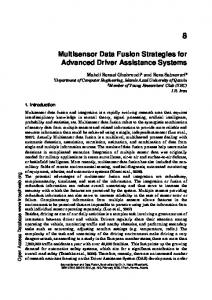
However, their spread is noticeably larger than the laser altimetry points, reflecting their lower precision. 6. Results 6.1. Extended time-series of dh/dt values We have determined with SERAC extended time-series at nine locations, numbered 1–9 in Fig. 1. Each of the sites is actually a surface patch, size 1 km × 1 km. Table 2 summarizes the most important results. SERAC employs a blunder detection/elimination scheme. In every iteration, the residuals are compared with the standard deviation and if their values exceed three times the standard deviation, the observation is flagged as a blunder and eliminated in the next iteration. This simple approach works well in our scenario of large redundancy and less than 10% blunders. The column number of epochs contains the number of time epochs per site. For example, site 8 has 30 different epochs, from single missions (e.g. topographic map, DISP, aerial photograph DEM) and repeat missions of ASTER and SPOT DEMs and laser altimetry. The last column of Table 2 lists σo, the square root of the unbiased estimation of unit variance. Considering the large redundancy, σo can be considered the error of fitting a 3rd order polynomial surface through the points (fitting error). We demonstrate the fusion aspect of SERAC with Fig. 7, a depiction of surface elevation change at site 5. The advantage of fusing various data sources in SERAC is evident: the time frame is greatly expanded

Table 2 Summary of SERAC computation at the nine sites marked in Fig. 1 with numbers 1–9. The second column contains the elevation of the site relative to the WGS-84 ellipsoid (note that the geoid height, i.e., local mean sea-level is 55.5 m in the Kangerlussuaq Fjord), at the reference time of August 31, 2006. The 3rd column lists the number of epochs, followed by the total number of points per site. The 5th column lists the number of blunders detected and eliminated and the last column contains the square root of the unbiased estimation of the unit variance. Site

1 2 3 4 5 6 7 8 9

Elevation

Number

Number

Number

σo

[m]

Epochs

Points

Blunders

[m]

883.74 770.25 770.97 851.28 370.86 174.84 164.92 1116.88 561.09

26 25 25 22 27 26 27 30 26

16,638 16,428 15,457 15,844 16,121 15,628 15,848 28,838 36,274

938 626 234 175 518 405 555 676 1838

7.40 5.70 6.23 3.66 4.47 7.46 5.93 6.01 4.18

back in time to 1933 and the sampling between 2000 to 2012 is densified. At site 5, the ice sheet was grounded for the entire duration of the record. Our reconstruction shows a gradual, slow lowering of the glacier's surface between 1933 and 2001 with an average rate of − 1.5±0.5 m a- 1. Thinning rates started to increase in 2001, reaching a maximum rate of 64 m a-1 in 2005. Thinning ceased abruptly in 2006. After a brief period of stability, the ice surface started to lower again in 2010 with an average thinning rate of 15 m a- 1 (Fig. 8, Site 5). Elevation change time-series reconstructed at sites 6 and 7, just upstream of the calving front, show similar patterns (Fig. 8). Note that the glacier at these sites might have started to float after the 2004–2005 retreat of the terminus and thinning episode. Further upstream, at site 2, thinning rates were lower and the glacier reached a new equilibrium later, consistent with a diffusive response to sudden thinning at the lower part of the drainage basin. 6.2. Correcting Stereoscopic DEMs As explained in detail in Section 5 the stereoscopic DEMs are corrected separately for systematic errors in planimetry and elevation (Eqs. (4–6)). We have applied a 2D similarity transformation to correct for the planimetric errors of the selected ASTER DEMs, using control points and control features (distinct lines identified and measured). The information about the vertical correction of the stereoscopic DEMs comes from the time-series of dh/dt points. A sigmoid curve is fitted through the more accurate laser altimetry points and the vertical differences from DEM points to the dispersion curve are the correction vectors. This leads to nine points in the DEMs through which we will fit a plane to determine the three unknown parameters of the vertical DEM correction. Table 3 lists the results. The table has 12 entries: 10 ASTER DEMs and 2 SPOT DEMs. The 3rd column, number points, refers to the number of sites that were used to determine the correction vector. The next three columns yield the correction parameters for the stereoscopic DEMs. The adjustment amounts to fitting a plane through the correction values (see Fig. 5). The two angular values, Δφ, Δω are in radians and must be multiplied with 10-4. Although the values are rather small, the angular adjustment has a fairly large impact. Taking an average value of Δφ = 5.10-4 and Δω =10.10-4 and considering the size of the test site (about 10 km × 25 km) gives an elevation difference at the margin of about 25 m due to angular errors only. The fitting error is the weighted square sum of residuals, divided by the number of points. Its average value of ±3.73 m for ASTER DEMs and ±2.06 m for SPOT indicates that there are no apparent modeling errors present, that is, for the small region of the test area, our linear, firstorder error model works well as long as we stay inside the boundary defined by SERAC points. 6.3. Calculation of elevation and volume changes Several previous studies employed ICESat and ATM laser altimetry observations and ASTER DEMs to investigate the rapid thinning that took place between 2003 and 2006 and to estimate the corresponding volume and mass loss (Howat et al., 2007, 2008; Thomas et al., 2009). However, altimetry measurements and stereoscopic DEMs were examined separately and thus provided reconstructions only along a few transects (altimetry) or had potentially large elevation errors in the ASTER DEMs. Here we present the first, detailed, accurate elevation change history of the lower part of the Kangerlussuaq drainage basin for 2001–2010, generated by fusing all topographic data. After the planimetric and the novel height adjustment of the DEMs we have selected six ASTER DEMs and one SPOT DEM that are more or less regularly distributed in time between the period 2001 to 2010 (dates marked by boldface numbers in Table 3). Fig. 9 shows the evolution of elevation change rates from 2001 to 2010 within the area enclosed by the yellow polygon in

T. Schenk et al. / Remote Sensing of Environment 149 (2014) 239–251

247

Fig. 7. Extended time-series ice sheet elevation change between 1933 and 2012 at site 5. Included in the glacier surface elevation change calculation are a digitized topographic map from 1933 with an estimated error of ±30 m, as well as a DEM derived from DISP with an estimated error of ±8 m. Other data sources (DEMs from stereo aerial photographs, ASTER and SPOT imagery; ATM laser altimetry data) have smaller error estimates – too small to be plotted in the figure.

Fig. 8. Detailed elevation change time-series showing the combined airborne laser altimetry and stereoscopic satellite DEM record since 1993. Sites are located along the central flowline of the Kangerlussuaq Glacier (sites 2, 5 and 6) and an additional site (7) near its calving front. Grey shaded area marks the period of abrupt retreat between July 1, 2004 and March 8, 2005.

248

T. Schenk et al. / Remote Sensing of Environment 149 (2014) 239–251

Table 3 Listed are the results of the ASTER and SPOT DEM correction. The 3rd column, number of points, is identical to the number of sites that gave the correction vector. The next three columns give the correction parameters for the stereoscopic DEMs. The two angular values, Δφ, Δω are in radians and must be multiplied with 10-4. The fitting error is the sum of the weighted square of residuals, divided by the number of points. Boldface numbers mark the dates of ASTER and SPOT DEMs used for computing annual or biannual elevation change rates shown in Fig. 9. Sensor

A S T E R

SP OT

Date

7/12/01 6/30/03 8/01/03 6/11/04 6/21/05 5/05/06 6/08/06 7/08/06 8/05/08 6/03/10 7/28n07 6/09/08

Num pts

9 9 9 6 9 9 9 9 9 9 9 7

Parameters

Fitting error

zT

Δφ

Δω

−5.39 3.86 0.01 16.13 3.51 17.54 17.24 25.84 12.90 0.24 7.98 1.16

4.00 −7.63 −0.64 −6.96 1.31 2.61 4.27 4.40 5.77 4.59 3.30 3.70

4.64 −7.04 4.78 18.40 0.52 6.35 14.79 11.13 3.65 6.55 4.69 1.27

3.72 2.34 2.83 2.76 3.37 4.85 5.92 4.45 4.25 2.78 2.33 1.78

Fig. 1. The uncorrected elevation change rates, presented in the upper row, show large temporal fluctuations, including tens of meters of thinning at higher elevations between 2003 and 2004, followed by a thickening with similar magnitude, as well as an abrupt, drainage basin-wide, short-term thickening in 2006–2007. Applying the corrections, we obtain a smooth sequence of elevation changes, depicting the diffusive response of the glacier to a rapid thinning near the grounding line. However, contrary to the expectations, this thinning of the lower region started in 2003–2004, i.e., prior to the retreat of the terminus. An early onset of thinning, starting in 2003, is also evident by examining the time-series in Fig. 8. Lower elevation thinning continued and intensified in 2004–2005, followed by a diffusive propagation of thinning toward the upper part of the drainage basin in 2005–2007.

Thinning rates decreased by 2007 when the fast flowing part of the glacier quickly adjusted to a new equilibrium state. Fig. 10 depicts the evolution of mass loss rates and the cumulative mass loss of the region between 2001 and 2010. We assumed that all mass loss was caused by ice dynamics and used an ice density of 917 kg m- 3. Errors were computed according to Rolstad, Haug, and Denby (2009), assuming that the DEM errors of about 6 m are not completely random, but correlated with a correlation length of 10 km. Mass loss represented by the gray dots and dashed polyline are obtained from the uncorrected DEMs while the black dots and solid polyline are the results from the corrected DEMs, including error bars of the mass changes. The evolution of mass loss rates shows a very good agreement with the modeled response of Jakobshavn Isbræ to a gradual retreat of its calving front (Vieli & Nick, 2011, Fig. 1). However, while the onset of acceleration and thinning of Jakobshavn Isbræ coincided to the break-up of its floating ice tongue, the Kangerlussaq Glacier has been thinning and loosing mass since 2003, when its calving front was still in a stable position. This suggests that rather than triggered by a calving front retreat, dynamic thinning of the Kangerlussuaq Glacier started when the lower section of the glacier reached floatation after slow thinning since 2001 (Thomas et al., 2009). Mass loss increased rapidly as the terminus retreated to the grounding line by Spring 2005. After a peak mass loss in 2005–2006, mass change rates quickly decreased. Since other authors reporting mass changes used different areas, we cannot directly compare our numbers. However, the shape of our final reconstruction of cumulative mass loss is in broad agreement with the changes reported by Howat et al. (2011), who also detected an accelerating mass loss between 2003 and 2006, followed by a gradual adjustment to a new equilibrium. 7. Discussion and error analysis We have presented a new approach for adjusting stereoscopic DEMs so that they optimally fit into the time-series of elevation changes with laser altimetry observations. Section 6 vividly demonstrated the

Fig. 9. Evolution of elevation change rates in the lower drainage basin of the Kangerlussuaq Glacier between 2001–2010. White line marks central flowline and white dots are sites used to register the ASTER DEMs, listed in Table 2. Dates of ASTER DEMs used to compute elevation change rates are marked by boldface numbers in Table 3. Upper row shows elevation change rates computed from uncorrected ASTER DEMs. Lower row is the result after applying the height adjustment derived from the altimetry record.

T. Schenk et al. / Remote Sensing of Environment 149 (2014) 239–251

249

Fig. 10. Mass change rates (left) and cumulative mass loss (right) of the lower part of the Kangerlussuaq drainage basin, shown in Fig. 9. Dashed polyline is computed from uncorrected ASTER DEMs, while solid polyline shows the final estimate of mass loss computed from the corrected ASTER DEMs with corresponding error bars. Grey shaded area marks the period of abrupt retreat between July 1, 2004 and March 8, 2005.

usefulness of this approach. The idea of combining stereoscopic DEMs with laser altimetry data is not new. For example, in Levinsen, Howat, and Tscherning (2013) the authors begin with pointing out the advantages of combining the data (sparse coverage, but accurate versus broad, if not continuous coverage, but less accurate DEMs). It is not clear, however, how the authors perform the co-registration of the DEMs to the laser point cloud, in absence of any known point to point correspondences. The focus of the paper is on geostatistical interpolation of residual differences between SPOT DEMs and laser altimetry. This statistical approach is rather different to our geometry based method. Kääb and Nuth have a number of publications about their experience with ASTER DEMs and suggest correction schemes (Kääb, 2005; Nuth & Kaab, 2011; Nuth, Moholdt, Kohler, Hagen, & Kaab, 2010). In essence, they propose to co-register ASTER DEMs to other DEMs, including ASTER DEMs of other time epochs by a mathematical approach that follows the observation that elevation differences and the aspect of the surface is related to the unknown shift vector between them. Their approach works well for DEMs that have enough stable ground and a distinct topography, for example large slopes pointing in all directions. Our scenario is different since our interest is the detection of elevation changes on large ice sheets and outlet glaciers – areas that lack a distinct topography and often times have very little stable terrain. Moreover, we need a good registration to laser altimetry point clouds. Throughout the paper we have included statements about accuracies and precision of our method. We now provide a summary. The leastsquares adjustment of SERAC produces not only unique values for the unknown parameters but also indicates their precision. The relevant observations are considered random variables, affected by random errors. Hence, the following discussion is based on the assumption that only random errors are present. SERAC determines elevation changes for a surface patch, not on spatially identical or near identical points. The surface is modeled by a polynomial, up to 3rd order. We make the assumption that surfaces at different times differ only in height but not in shape. The adjustment delivers the shape parameters and, more important, the height at the time epochs (absolute elevation). The precision of the absolute elevations is of prime interest as this gives the error bars for the points in the timeseries. It is obtained from the diagonal elements, also known as cofactors, of the variance-covariance matrix (inverse of normal equation matrix), multiplied with σo. While the co-factors largely depend on the geometry of the adjustment problem, σo is related to the precision of the observations.

Let us now examine the values of σo a bit further. Recalling that SERAC models the surface patch (here 1 km × km) by a third order polynomial and considering that the real surface in this part of the Kangerlussuaq Glacier is much more rugged than a 3rd order polynomial is able to capture, we conclude that σo is affected by the modeling error – an error due to a insufficient (or wrong) mathematical model. How can we estimate the modeling error and correct σo so that it reflects more closely the error of the weighted observations? Assume for a moment that we divide the data sets into laser altimetry points and stereoscopic DEM points and run SERAC again. We did this, except we selected 10 ASTER DEMs within the time span 2001–2010, giving an average of σo = ±2.03 m for the laser altimetry points, a much higher value than we would expect from the point precision and number of points. Therefore we consider ±2.00 m as an average modeling error. The resulting σo for running SERAC with the 10 selected ASTER DEMs was on average ± 6.44 m. Subtracting the modeling error gives σo = ±6.07 m – a more realistic estimate for the precision of the corrected ASTER DEMs. With the adjusted σo values we can now determine the precision of the computed surface elevation per time epoch. For the ASTER DEMs we find an average value of ±0.18 m. The low value may come as a surprise but we should not forget pthat ffiffiffiffiffiffiffiffiffiffiffiabout 1100 points contribute to one epoch and multiplying 0:18 1100 ¼ 6:3 m is about the average height precision of an ASTER DEMs grid post. The same calculation for laser altimetry points renders an average precision of ±0.01 m. 8. Conclusions and outlook Cryospheric research, such as mass balance studies and related estimates of sea-level rise, greatly benefit from information about surface elevation changes and annual change rates. There is an increased interest in the modeling community to using surface elevation and change rates directly with other information, such as velocities, in assimilation models. Until now, surface elevation changes have been determined from repeat laser altimetry data, both, from aerial and space platforms. While the precision of laser altimetry data is high (single shot accuracy a few decimeter), the spatial coverage is scarce because the samples of change rates are confined to repeat ground tracks. In areas of rapid changes, such as outlet glaciers, denser sampling is needed. Our new method enables the reconstruction of spatio-temporal evolution of rapidly changing outlet glaciers with unprecedented details. Such reconstructions are especially valuable for investigating the roles that different environmental forcings play in the sudden dynamic changes

250

T. Schenk et al. / Remote Sensing of Environment 149 (2014) 239–251

of outlet glaciers, a key to improving prognostic models of ice sheet evolution and sea level rise. Stereoscopic DEMs derived from repeat space imagery gives an almost continuous coverage but the accuracy is at least one order of magnitude larger than laser altimetry. It makes sense to fuse these disparate data sets in order to extend the time-series of elevation changes back in time and to increase the spatial density. We have presented a novel method to fuse data sets from widely different sources, such as a digitized topographic map from 1933, stereoscopic DEMs from the 1960s (DISP), 1980s (aerial images), laser altimetry data from ATM (1993–2012), LVIS (2008–2012), ICESat (2003–2009), and stereoscopic DEMs from ASTER and SPOT. After co-registering the various data sets to the WGS84 ellipsoidal reference system, the data have been entered into SERAC with its unique property of determining surface elevation changes between small surfaces, rather than between identical or near identical points. This leads to a consistent time-series of surface elevation and allows easy calculation of annual change rates. Our novel method for correcting stereoscopic DEMs is rooted in the time-series of surface elevation changes calculated by SERAC. A perturbation of a glacier causes a response of the surface that can be well approximated by a sigmoid curve. Fitting a sigmoid curve to the more accurate laser altimetry points of the time-series reveals that the DEM points are systematically displaced from the curve. We use these systematic errors as observations for the height adjustment of the DEMs. The adjustment has three unknowns: shift in height and two angles, about which the DEM is rotated in space. The results clearly demonstrate that the introduction of the two angles greatly improves the correction of the DEMs. An important question we will address in future research is the validity of the linear height transformation. There is ample evidence of remaining systematic errors that cause a deformation of the DEMs. However, it is difficult to rationalize or even model these errors, partially because the rational function models (RFM), given by the providers of satellite images, do not have sufficient information about important camera details, calibration procedures and how an image is formed from individual lines of push-broom systems. Finally, this study used a simple sigmoid curve to approximate elevation changes caused by a single perturbation, for example rapid thinning near the grounding line. Reconstructing longer time histories might require the modeling of more complicated temporal evolutions. Acknowledgements We acknowledge Henry Brecher for computing the aerial photogrammetry DEM, Yushin Ahn for converting the topographic map into a DEM, and Greg Babonis for help with altimetry processing. Authors acknowledge support by the National Aeronautics and Space Administrations Polar Program under Grants NNX10AV13G (Operation IceBridge) and NNX11AR23G. References Abdalati, W., Krabill, W., Frederick, E., Manizade, S., Martin, C., Sonntag, J., et al. (2002). Airborne laser altimetry mapping of the Greenland ice sheet: application to mass balance assessment. Journal of Geodynamics, 34, 391–403. Abrams, M. (2000). The Advanced Spaceborne Thermal Emission and Reflection Radiometer (ASTER): data products for the high spatial resolution imager on NASA’s Terra platform. International Journal of Remote Sensing, 21, 847–859. Alley, R. B., Clark, P. U., Huybrechts, P., & Joughin, I. (2005). Ice-sheet and sea-level changes. Science, 310, 456–460. Bjørk, A. A., Kjær, K. H., Korsgaard, N. J., Khan, S. A., Kjeldsen, K. K., Andresen, C. S., et al. (2012). An aerial view of 80 years of climate-related glacier fluctuations in southeast Greenland. Nature Geoscience, 5, 427–432. Blair, J. B., Rabine, D. L., & Hofton, M. A. (1999). The Laser Vegetation Imaging Sensor: a medium-altitude, digitisation-only, airborne laser altimeter for mapping vegetation and topography. ISPRS Journal of Photogrammetry and Remote Sensing, 54, 115–122. Borsa, A. A., Moholdt, G., Fricker, H. A., & Brunt, K. M. (2013). A range correction for ICESat and its potential impact on ice sheet mass balance studies. The Cryosphere Discussions, 7, 4287–4319.

Bouillon, A., Bernard, M., Gigord, P., Orsoni, A., Rudowski, V., & Baudoin, A. (2006). SPOT 5 HRS geometric performances: Using block adjustment as a key issue to improve quality of DEM generation. ISPRS Journal of Photogrammetry and Remote Sensing, 60, 134–146. Csatho, B.M., Bolzan, J. F., Van Der Veen, C. J., Schenk, A. F., & Lee, D. C. (1999). Surface velocities of a Greenland outlet glacier from high-resolution visible satellite imagery 1. Polar Geography, 23, 71–82. Csatho, B., Schenk, A., Duncan, K., Babonis, G., Sonntag, J., Krabill, W., et al. (2013). Greenland Ice Sheet Mass Loss and Outlet Glacier Dynamics from Laser Altimetry Record. Abstract C53D-02 presented at 2013 Fall Meeting, AGU, San Francisco, Calif., 9-13 Dec. 2013. Csatho, B., Schenk, T., Shin, S. W., & Van Der Veen, C. J. (2002). Investigating long-term behavior of Greenland outlet glaciers using high resolution satellite imagery. IEEE Geoscience and Remote Sensing Symposium, IGARSS’02 (pp. 1047–1050). Csatho, B., Schenk, T., Van Der Veen, C. J., & Krabill, W. B. (2008). Intermittent thinning of Jakobshavn Isbræ, West Greenland, since the Little Ice Age. Journal of Glaciology, 54, 131–144. Domack, E., Duran, D., Leventer, A., Ishman, S., Doane, S., McCallum, S., et al. (2005). Stability of the Larsen B ice shelf on the Antarctic Peninsula during the Holocene epoch. Nature, 436, 681–685. Fricker, H. A. (2005). Assessment of ICESat performance at the salar de Uyuni, Bolivia. Geophysical Research Letters, 32, L21S06. Fujisada, H., Baily, G., Kelly, G., Hara, S., & Abrams, M. (2005). ASTER DEM performance. Journal of Remote Sensing, IEEE, 43, 2707–2714. Gabel-Jorgensen, C. A. A. (1935). Dr. Knud Rasmussens contribution to the exploration of the south-east coast of Greenland, 1931–1933. Journal of Geography, 86, 32–49. Hofton, M.A., Blair, J. B., Luthcke, S. B., & Rabine, D. L. (2008). Assessing the performance of 20–25 m footprint waveform LIDAR data collected in ICESat data corridors in Greenland. Geophysical Research Letters, 35. Howat, I. M., Ahn, Y., Joughin, I., Van Den Broeke, M. R., Lenaerts, J. T. M., & Smith, B. (2011). Mass balance of Greenland’s three largest outlet glaciers, 2000–2010. Geophysical Research Letters, 38, L12501. Howat, I. M., Joughin, I., & Scambos, T. A. (2007). Rapid changes in ice discharge from Greenland outlet glaciers. Science, 315, 1559–1561. Howat, I. M., Smith, B. E., Joughin, I., & Scambos, T. A. (2008). Rates of southeast Greenland ice volume loss from combined ICESat and ASTER observations. Geophysical Research Letters, 35, L17505. Iwasaki, A., & Fujisada, H. (2005). ASTER geometric performance. Journal of Remote Sensing, IEEE, 43, 2700–2706. Kääb, A. (2005). Remote sensing of mountain glaciers and permafrost creep. Geographisches Institut der Universität Zürich. Kerekes, J., Goodenough, A., Brown, S., Zhang, J., Csatho, B., Schenk, T., et al. (2012). First principles modeling for LIDAR sensing of complex ice surfaces. IEEE International Geoscience and Remote Sensing Symposium (pp. 3241–3244). Koenig, H. J., Martin, S., Studinger, M., & Sonntag, J. (2011). Polar airborne observations fill gap in satellite data. American Geophysical Union, Eos Transactions, 91, 333–334. Korona, J., Berthier, E., Bernard, M. R. F., & Thouvenot, E. (2009). SPIRIT. SPOT 5 stereoscopic survey of Polar Ice: reference images and topographies during the fourth International Polar Year (2007–2009). ISPRS Journal of Photogrammetry and Remote Sensing, 64, 204–221. Krabill, W. B., Abdalati, W., Frederick, E. B., Manizade, S. S., Martin, C. F., Sonntag, J. G., et al. (2002). Aircraft laser altimetry measurement of elevation changes of the Greenland ice sheet: Technique and accuracy assessment. Journal of Geodynamics, 34, 357–376. Levinsen, J. F., Howat, I. M., & Tscherning, C. C. (2013). Improving maps of ice-sheet surface elevation change using combined laser altimeter and stereoscopic elevation model data. Journal of Glaciology, 59, 524–532. Martin, C. F., Krabill, W. B., Manizade, S. S., & Russell, R. L. (2012). Airborne topographic mapper calibration procedures and accuracy assessment. NASA Technical Memorandum, 2012–215891. McDonald, R. (1995). Opening the cold war to the public: declassifying satellite reconnaissance imagery. Photogrammetric Engineering and Remote Sensing, 61, 385–390. McDonald, R. (1997). Corona between the Sun and the Earth. American Society of Photogrammetry and Remote Sensing, 5410 Grosvenor Lane, Bethesda, MD. Moon, T., Joughin, I., Smith, B., & Howat, I. (2012). 21st-century evolution of Greenland outlet glacier velocities. Science, 336, 576–578. Nick, F., Vieli, A., Andersen, L., Joughin, I., Payne, A., Edwards, T., et al. (2013). Future sea-level rise from Greenland’s main outlet glaciers in a warming climate. Nature, 497, 235–238. Nuth, C., & Kääb, A. (2011). Co-registration and bias corrections of satellite elevation data sets for quantifying glacier thickness change. The Cryosphere, 5, 271–290. Nuth, C., Moholdt, G., Kohler, J., Hagen, J. O., & Kääb, A. (2010). Svalbard glacier elevation changes and contribution to sea level rise. Journal of Geophysical Research, 115, F01008. Price, S. F., Payne, A. J., Howat, I. M., & Smith, B. E. (2011). Committed sea-level rise for the next century from Greenland ice sheet dynamics during the past decade. Proceedings of the National Academy of Sciences, 108, 8978–8983. Pritchard, H. D., Arthern, R., Vaughan, D.G., & Edwards, L. A. (2009). Extensive dynamic thinning on the margins of the Greenland and Antarctic ice sheets. Nature, 461, 971–975. Rignot, E., Velicogna, I., Van Den Broeke, M. R., Monaghan, A., & Lenaerts, J. (2011). Acceleration of the contribution of the Greenland and Antarctic ice sheets to sea level rise. Geophysical Research Letters, 38, L05503. Rolstad, C., Haug, T., & Denby, B. (2009). Spatially integrated geodetic glacier mass balance and its uncertainty based on geostatistical analysis: application to the western Svartisen ice cap, Norway. Journal of Glaciology-Only, 55, 666–680.

T. Schenk et al. / Remote Sensing of Environment 149 (2014) 239–251 Schenk, T. (1999). Digital photogrammetry. TerraScience, 16218 Bailor Rd., Laurelville, OH 43135. Schenk, T., & Csatho, B. (2012). A new methodology for detecting ice sheet surface elevation changes from laser altimetry data. IEEE Transactions on Geoscience and Remote Sensing, 50, 3302–3316. Schenk, T., Csatho, B., & Shin, S. W. (2003). Rigorous panoramic camera model for DISP imagery. Proceedings of Joint Workshop of ISPRS Working Groups I/2, I/5, IC WG II/IV and EARSeL Special Interest Group: 3D Remote Sensing, High Resolution Mapping from Space 2003 (pp. 1–6) TU Hannover, Hannover, Germany. Schenk, T., Csatho, B., Van Der Veen, C. J., Brecher, H., Ahn, Y., & Yoon, T. (2005). Registering imagery to ICESat data for measuring elevation changes on Byrd Glacier, Antarctica. Geophysical Research Letters, 32, L23S0. Schutz, B. E., Zwally, H. J., Shuman, C. A., Hancock, D., & Dimarzio, J. P. (2005). Overview of the ICESat Mission. Geophysical Research Letters, 32, L21S01. Shepherd, A., Ivins, E. R., Barletta, V. R., Bentley, M. J., & Bettadpur, S. (2012). A reconciled estimate of ice-sheet mass balance. Science, 338, 1183–1189. Shuman, C. A., Zwally, H. J., Schutz, B. E., Brenner, A.C., Dimarzio, J. P., Suchdeo, V. P., et al. (2006). ICESat Antarctic elevation data: Preliminary precision and accuracy assessment. Geophysical Research Letters, 33, L07501. Sutterly, T., Velicogna, I., Csatho, B., van den Broeke, M., Rezvan-Behbahani, S., & Babonis, G. (2013). Evaluating Greenland glacial isostatic adjustment correction using GRACE, altimetry and surface mass balance data. Environmental Research Letters, 9, 9pp (014004). Thomas, R. H., Abdalati, W., Akins, T. L., Csathó, B.M., Frederick, E. B., Gogineni, S. P., et al. (2000). Substantial thinning of a major east Greenland outlet glacier. Geophysical Research Letters, 27, 1291–1294.

251

Thomas, R., Frederick, E., Krabill, W., Manizade, S., & Martin, C. (2009). Recent changes on Greenland outlet glaciers. Journal of Glaciology, 55, 147–162. Toutin, T. (2004). Comparison of stereo-extracted DTM from different high-resolution sensors: SPOT-5, EROS-A, IKONOS-II, and QuickBird. IEEE transactions on geoscience and remote sensing, 42, 2121–2129. Toutin, T. (2008). ASTER DEMs for geomatic and geoscientific applications: a review. International Journal on Remote Sensing, 29, 1855–1875. Van Der Veen, C. J., Ahn, Y., Csatho, B.M., Mosley-Thompson, E., & Krabill, W. B. (2009). Surface roughness over the northern half of the Greenland Ice Sheet from airborne laser altimetry. Journal of Geophysical Research, 114, F01001. Van Der Veen, C. J., Krabill, W. B., Csatho, B.M., & Bolzan, J. F. (1998). Surface roughness on the Greenland ice sheet from airborne laser altimetry. Geophysical Research Letters, 25, 3887–3890. Vieli, A., & Nick, F. M. (2011). Understanding and modelling rapid dynamic changes of tidewater outlet glaciers: issues and implications. Surveys in Geophysics, 32, 437–458. Wingham, D. J., Wallis, D. W., & Shepherd, A. (2009). Spatial and temporal evolution of Pine Island Glacier thinning, 1995–2006. Geophysical Research Letters, 36, L17501. Wolf, P., & Dewitt, B. (2000). Elements of photogrammetry. McGraw-Hill. Zwally, H. J., Jun, L. I., Brenner, A.C., Beckley, M., Cornejo, H. G., Dimarzio, J., et al. (2011). Greenland ice sheet mass balance: distribution of increased mass loss with climate warming; 2003–07 versus 1992–2002. Journal of Glaciology, 57, 88–102. Zwally, H. J., Schutz, B., Abdalati, W., Abshire, J., Bentley, C., Brenner, A., et al. (2002). ICESat’s laser measurements of polar ice, atmosphere, ocean, and land. Journal of Geodynamics, 34, 405–445.