Hindawi Publishing Corporation Discrete Dynamics in Nature and Society Volume 2016, Article ID 5704743, 14 pages http://dx.doi.org/10.1155/2016/5704743
Research Article Fuzzy Constrained Predictive Optimal Control of High Speed Train with Actuator Dynamics Xi Wang,1 Yan Zhao,2 and Tao Tang3 1
National Engineering Research Center of Rail Transportation Operation and Control System, Beijing Jiaotong University, Beijing, China 2 Advanced Control Systems Lab of the School of Electronic and Information Engineering, Beijing Jiaotong University, Beijing, China 3 State Key Laboratory of Rail Traffic Control and Safety, Beijing Jiaotong University, Beijing, China Correspondence should be addressed to Xi Wang;
[email protected] Received 2 June 2016; Accepted 17 August 2016 Academic Editor: Manuel De la Sen Copyright © 2016 Xi Wang et al. This is an open access article distributed under the Creative Commons Attribution License, which permits unrestricted use, distribution, and reproduction in any medium, provided the original work is properly cited. We investigate the problem of fuzzy constrained predictive optimal control of high speed train considering the effect of actuator dynamics. The dynamics feature of the high speed train is modeled as a cascade of cars connected by flexible couplers, and the formulation is mathematically transformed into a Takagi-Sugeno (T-S) fuzzy model. The goal of this study is to design a state feedback control law at each decision step to enhance safety, comfort, and energy efficiency of high speed train subject to safety constraints on the control input. Based on Lyapunov stability theory, the problem of optimizing an upper bound on the cruise control cost function subject to input constraints is reduced to a convex optimization problem involving linear matrix inequalities (LMIs). Furthermore, we analyze the influences of second-order actuator dynamics on the fuzzy constrained predictive controller, which shows risk of potentially deteriorating the overall system. Employing backstepping method, an actuator compensator is proposed to accommodate for the influence of the actuator dynamics. The experimental results show that with the proposed approach high speed train can track the desired speed, the relative coupler displacement between the neighbouring cars is stable at the equilibrium state, and the influence of actuator dynamics is reduced, which demonstrate the validity and effectiveness of the proposed approaches.
1. Introduction High speed railway systems have attracted much attention, since they can provide greater transport capacity, significantly faster speeds, and outstanding features of punctuality when compared to aircraft and autovehicle. In recent years, high speed railways have gone through rapid development in European countries, Russia, Japan, China, and many other developing countries. As the high speed railways networks are becoming more and more complex, many new challenging technical and commercial issues such as reduction of energy consumption, safety, and comfort have been brought up. With the breakthrough in computer control and communication technology, the automatic train control (ATC) system is equipped to automatically supervise the train speed to follow a desired trajectory which also makes it possible to adjust the train operations in a safe and energy-efficient way [1–3].
Many scholars and researchers have therefore been searching for the optimal driving strategy over the years. Howlett [4] applied the Pontryagin maximum principle to prove that the optimal sequence of train driving strategy should consist of four phases including maximum acceleration, cruising, coasting, and maximum braking [4–6]. Therefore, the train driving problem is characterized by the switching locations of stages which can be formally formulated as a nonlinear optimization problem. Furthermore, various algorithms were proposed to determine the optimal cruising speed and the switching locations, for example, genetic algorithm [7], ant colony optimization method [8], and simulated annealing algorithm [9], considering the realworld operation environments such as track gradient and speed limits, commercial punctuality constraints, and the uncertainty of some performance parameters [10, 11].
2 It should be clarified that above methods for automatic train control treated the whole train that consists of multiple cars as a single point mass and approximately characterized its motion by a single mass point Newton equation. Although the single mass point model makes design of the controller much convenient, it overlooks the interactive forces among the connected vehicles which should be explicitly contemplated to achieve satisfactory control performance for a long train. In order to overcome these disadvantages, Gruber and Bayoumi [12] investigated the longitudinal dynamics of multilocomotive powered train and approximated it as a nonlinear mass-spring dashpot model which was interconnected via couplers at the first time. They demonstrated that this method could efficiently minimize the coupler forces which result in safer operation and increased traveling speeds. Zhuan and Xia [13] obtained an open-loop scheduling controller by solving an optimization problem based on the desired trajectory, and closed-loop controller was subsequently presented through local linearization to maintain a steady-state motion of a train [14]. Song et al. [15] extended the cascade mass point to model the high speed train under unknown and time varying resistance coefficients and designed robust adaptive control with optimal task distribution for speed and position tracking with traction/braking nonlinearities and saturation limitations. As the aerodynamic resistance is proportional to the square of the train’s speed, the most typical way to handle this case is to linearize or approximate the impacts along a prior scheduled ideal speed [16–18]. Although this approach simplifies computational complexity, its influence on the train’s dynamic behavior becomes increasingly significant as the train speed increases. As a popular control method, the fuzzy logic control has been developing quickly during the past thirty years, where prevailing attention has been devoted to Takagi-Sugeno (T-S) fuzzy model based control for complex nonlinear systems [19–21]. Taking fuzzy control methods and optimization techniques as alternatives, many research works have been done in the high speed train control and optimization fields [22–24]. However, it is worth noting that most existing methods for high speed train control focus on optimizing the operation of a high speed train according to the current information, and future behaviors during the whole travel are usually not taken into consideration. Therefore, these approaches cannot ensure an overall optimized operation of the train during a long trip due to the unfavorable factors such as model inaccuracies, operation constraints, and uneven track profile [25, 26]. As one of the most powerful directions of the modern control, model predictive control (MPC) can be regarded as a circular operation in which a minimization problem is solved to calculate optimal control for certain time horizon with hard physical constraints [27, 28]. This feature makes MPC an ideal candidate for optimal cruise control of high speed train too. Moreover, most approaches of high speed train controller design assume that traction/braking dynamics are fast enough to be negligible. However, it turns out that actuators show limited performance in real situations and, accordingly, the control performance would be severely degraded if we design the traction/braking force for the train directly.
Discrete Dynamics in Nature and Society Motivated by earlier discussions, the main purpose of this brief is to solve the high speed controller optimization problem which guarantees the various railway operational performances such as safety, energy consumption, riding comfort, and velocity tracking with explicit consideration of input constraints as well as the actuator dynamics. Different from the existing results [18, 29], in this paper, T-S fuzzy model which provides a bridge between the analysis of nonlinear systems and the fruitful linear control theory is employed to approximate the nonlinear dynamic model of high speed train. Instead of using conventional open-loop model prediction, this brief proposes a fuzzy constrained predictive controller using a state feedback control scheme to facilitate a finite dimensional formulation for an infinite horizon in closed-loop prediction form. The asymptotical stability and controller synthesis can be explicitly formulated as a convex optimization problem in which the related sufficient conditions of stability are cast into a set of linear matrix inequalities (LMIs) based on Lyapunov function. Furthermore, we analyze the influence of actuator dynamics on the fuzzy constrained predictive controller and design a compensator using backstepping technique [30] to accommodate for the influence of the actuator. The remainder of this research is organized as follows. Section 2 details the T-S fuzzy model that preserves the nonlinear nature of the high speed train dynamics while, at the same time, facilitating the control design. In Section 3, the fuzzy constrained predictive controller of high speed train is designed and the compensator scheme based on backstepping is introduced. The numerical experiments are implemented in Section 4 for demonstrating the validity and effectiveness of the proposed approaches. Finally, some conclusions and further works are addressed in Section 5. Some notations are given as follows: (1) The symbol ∗ in a matrix will be used in the subsequent sections to stand for the corresponding item of a symmetric matrix. (2) 𝑥(𝑘 + 𝑗 | 𝑘) is the predicted state at time 𝑘 + 𝑗 based on the current state 𝑥(𝑘).
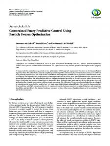
2. Problem Formulation 2.1. The Dynamic Model of High Speed Train. Consider a high speed train consisting of 𝑛 cars, which is modeled by a cascade of cars connected with flexible couplers. As mentioned in [16, 31], the behavior of couplers is described approximately by linear spring with stiffness coefficient 𝑘. Therefore, the intrain force is described approximately by a linear function of the coupler relative displacement 𝑥 between two adjacent cars, which can be established as follows: 𝑓 (𝑥) = 𝑘𝑥𝑖 , 𝑖 = 1, 2, . . . , 𝑛 − 1.
(1)
As 𝑥𝑖 represents the absolute extension or compression length of the 𝑖th coupler corresponding to the original length without any elastic deformation, it could be positive or negative.
Discrete Dynamics in Nature and Society Car n
3
Car n − 1
fn−1 Coupler n − 1
···
Coupler n − 2
un Rmn
Car 2 fn−2
Car 1
f1
f2 Coupler 2
Coupler 1
u2
un−1 Rm(n−1)
Ra
u1 Rm1
Rm2
Figure 1: Longitudinal dynamics of high speed train.
The force diagram of high speed train is depicted in Figure 1, where 𝑢𝑖 , 𝑅𝑚𝑖 , and 𝑅𝑎 denote traction force, mechanical resistance, and aerodynamic drag of the 𝑖th car, respectively. Let 𝑚𝑖 be the mass of 𝑖th car; then according to Davis’ equation [32], 𝑅𝑚𝑖 and 𝑅𝑎 are given by
To study the cruise control problem of the high speed train, the desired cruise speeds for each car of the high speed train are supposed as V∗ and the relative coupler displacements between the connected cars are 𝑥∗ which is equal to zero at the equilibrium state. Then the control forces in the equilibrium state are calculated as
𝑅𝑚𝑖 = (𝑐0 + 𝑐1 V𝑖 ) 𝑚𝑖 ,
𝑢1 = (𝑐0 + 𝑐1 V∗ ) 𝑚1 + 𝑐2 (∑𝑚𝑖 ) (V∗ ) ,
𝑛
(2)
𝑅𝑎 = 𝑐2 𝑀V𝑖2 ,
𝑖=1
∗
𝑢𝑖 = (𝑐0 + 𝑐1 V ) 𝑚𝑖 ,
where 𝑐0 , 𝑐1 , and 𝑐2 are positive constants and 𝑀 is the total mass of train given by ∑𝑛𝑖=1 𝑚𝑖 . We assume that the air resistance acts only on the leading car and the rolling resistance acts on every car. According to Newton’s law, the longitudinal dynamics for each car can be established by the following equation:
2
𝑖 = 2, 3, . . . , 𝑛 − 1.
̂ 𝑖 = 𝑢𝑖 −𝑢𝑖 and chooŝ 𝑖 = 𝑥𝑖 −𝑥∗ , ̂V𝑖 = V𝑖 −V∗ , and 𝑢 Letting 𝑥 ̂ 2 (𝑡), . . . , 𝑥 ̂ 𝑛−1 (𝑡), ̂V1 (𝑡), ̂V2 (𝑡), . . . , ̂V𝑛 (𝑡)]𝑇 ing 𝑥(𝑡) = [̂ 𝑥1 (𝑡), 𝑥 ̂ 2 (𝑡)/𝑚2 , . . ., as the state variable and 𝑢(𝑡) = [̂ 𝑢1 (𝑡)/𝑚1 , 𝑢 ̂ 𝑛 (𝑡)/𝑚𝑛 ]𝑇 as the decision vector, the error dynamic equation 𝑢 around the equilibrium state can be formulated as 𝑥̇ (𝑡) = 𝐴𝑥 (𝑡) + 𝐵𝑢 (𝑡) ,
𝑚1 V̇1 = 𝑢1 − 𝑓1 − 𝑅𝑚1 − 𝑅𝑎 ,
(6)
where
𝑚𝑖 V̇𝑖 = 𝑢𝑖 + 𝑓𝑖−1 − 𝑓𝑖 − 𝑅𝑚𝑖 , 𝑖 = 2, 3, . . . , 𝑛,
(3)
where 𝑚𝑖 is the inertia mass, V𝑖 is the speed of the 𝑖th car, and 𝑓𝑖 denotes the interactive force between the 𝑖th car and the (𝑖 + 1)th car. To achieve the high-precise velocity tracking, it is assumed that every car of the high speed train has its own independent control command, and we will adopt the distributed driving design for each car of the high speed train. Then the dynamic equation of an 𝑛-cars high speed train can be obtained from (1) to (3) that 𝑥̇ 𝑖 (𝑡) = V𝑖 − V𝑖+1 ,
(5)
𝐴 11 𝐴 12 𝐴=[ ], 𝐴 21 𝐴 22 1 −1 0 0 ⋅ ⋅ ⋅ ] [ 𝐴 12 = [0 1 −1 0 ⋅ ⋅ ⋅]
,
[0 ⋅ ⋅ ⋅ 0 1 −1](𝑛−1)×𝑛
𝐴 21
𝑘 0 [− 𝑚 [ 1 [ 𝑘 𝑘 [ [ 𝑚 −𝑚 2 2 =[ [ [ 0 ⋅⋅⋅ [ [ [ 0 ⋅⋅⋅ [
0
⋅⋅⋅
0
⋅⋅⋅
0
𝑘 𝑚𝑛−1
0
0
0
] ] ] 0 ] ] ] , 𝑘 ] ] − ] 𝑚𝑛−1 ] 𝑘 ] 𝑚𝑛 ]𝑛×(𝑛−1)
𝐴 22
𝑖 = 1, 2, . . . , 𝑛,
𝑛
𝑛
𝑚1 V̇1 (𝑡) = 𝑢1 − 𝑘𝑥1 − (𝑐0 + 𝑐1 V1 ) 𝑚1 − 𝑐2 (∑𝑚𝑖 ) V12 , 𝑖=1
𝑚𝑖 V̇𝑖 (𝑡) = 𝑢𝑖 + 𝑘𝑥𝑖−1 − 𝑘𝑥𝑖 − (𝑐0 + 𝑐1 V𝑖 ) 𝑚𝑖 , 𝑖 = 2, 3, . . . , 𝑛 − 1, 𝑚𝑛 V̇𝑛 (𝑡) = 𝑢𝑛 + 𝑘𝑥𝑛−1 − (𝑐0 + 𝑐1 V𝑛 ) 𝑚𝑛 .
(4)
(∑𝑖=1 𝑚𝑖 ) (̂V1 + 2V∗ ) 𝑚1 𝑐1 0 0 ⋅⋅⋅ 0 ] [− 𝑚 − 𝑐2 𝑚1 [ ] 1 𝑚2 𝑐1 [ ] =[ 0 − 0 ⋅⋅⋅ 0 ] , [ ] 𝑚 2 [ 𝑚 𝑐 ] 0 ⋅⋅⋅ 0 0 − 𝑛 1 𝑚𝑛 ]𝑛×𝑛 [ 𝐴 11 = 0(𝑛−1)×(𝑛−1) , 𝑇
𝐵 = [0𝑛×(𝑛−1) , 𝐼𝑛×𝑛 ] .
(7)
4
Discrete Dynamics in Nature and Society
In order to apply the MPC framework, the continuous time-domain state-space equation (6) is discretized by the zero-order hold method with a sampling period 𝑇𝑠 : 𝑥 (𝑘 + 1) = 𝐴𝑥 (𝑘) + 𝐵𝑢 (𝑘) ,
(8)
𝑇
where 𝐴 = 𝑒𝐴𝑇𝑠 and 𝐵 = ∫0 𝑠 𝑒𝐴𝜏 𝑑𝜏𝐵. 2.2. T-S Fuzzy Model for the High Speed Train. It has been proven that T-S fuzzy models can approximate any smooth nonlinear system to any accuracy within a compact set. The following T-S fuzzy dynamic model proposed in [19, 33] can be used to represent the high speed train with both fuzzy inference rules and local analytic linear models as follows: Fuzzy rule 𝑙: IF ̂V1 (𝑘) is 𝑀1𝑙 and ⋅ ⋅ ⋅ and ̂V𝑛 (𝑘) is 𝑀𝑛𝑙 , THEN 𝑥 (𝑘 + 1) = 𝐴 𝑙 𝑥 (𝑘) + 𝐵𝑙 𝑢 (𝑘) ,
𝑙 = 1, . . . , 𝑟.
(9)
Here, 𝑟 is the number of inference rules and 𝑀𝑖𝑙 (𝑖 = 1, 2, . . . , 𝑛) are the fuzzy sets; 𝑥(𝑘) is the state vector and 𝑢(𝑘) is the input vector, both of which are defined in (8); 𝐴 𝑙 and 𝐵𝑙 are known constant matrices with appropriate dimensions. Let ℎ𝑙 (𝑧(𝑘)) be the normalized membership function of the inferred fuzzy set 𝑀𝑙 , where 𝑧(𝑘) = [̂V1 (𝑘), . . . , ̂V𝑛 (𝑘)], 𝑀𝑙 = ∏𝑛𝑖=1 𝑀𝑖𝑙 , and ∑𝑟𝑙=1 ℎ𝑙 (𝑧(𝑘)) = 1. By using a centeraverage defuzzifier, product inference, and singleton fuzzifier, the dynamic fuzzy model (9) can be expressed by the following global model:
Remark 1. In the optimization objective criterion (11), the deviations of relative coupler displacements for each car are defined as the indicators of safety and riding comfort. Generally speaking, the integrand 𝑢𝑖 (𝑡)V𝑖 (𝑡) represents the exported tractive power of train 𝑖 at time 𝑡. Since our attention is focused on the energy consumption associated with the control strategy tending to the equilibrium state, we use the second part to express the energy efficiency performance. The third term represents the error of tracking the desired speed profile. One of the most appealing features of the MPC is that the transient control performance of the closed-loop system can be adequately addressed in terms of certain optimal performance cost. For the train operation problem, the fuzzy constrained MPC approach uses the current train dynamic state, train model, and operational limits to compute future control inputs, so that the train operating performance (11) is optimized over the prediction horizon. Assume that exact measurement of the train state 𝑥(𝑘 | 𝑘) is available at each sampling decision step 𝑘, and let 𝑥(𝑘+𝑗 | 𝑘) be the predicted state of the high speed train at time 𝑘 + 𝑗 and let 𝑢(𝑘 + 𝑗 | 𝑘) be the future control at time 𝑘 + 𝑗; we consider the infinite horizon MPC problem with a quadratic objective as [34]. According to the error dynamical equation (8), the above performance objective function can be mathematically transformed into the following optimization problem: min
𝑢(𝑘+𝑗|𝑘)
𝐽0∞ (𝑘) 𝑇 (12) 𝑥 (𝑘 + 𝑗 | 𝑘) 𝑄 0 𝑥 (𝑘 + 𝑗 | 𝑘) ][ ], ] [ = ∑[ 0 𝑅 𝑢 (𝑘 + 𝑗 | 𝑘) 𝑗=0 𝑢 (𝑘 + 𝑗 | 𝑘) ∞
where
𝑟
𝑥 (𝑘 + 1) = ∑ℎ𝑙 (𝑧 (𝑘)) (𝐴 𝑙 𝑥 (𝑘) + 𝐵𝑙 𝑢 (𝑘)) , 𝑙=1
(10)
𝑙 = 1, . . . , 𝑟.
3. Optimal Cruise Control Design The goal of the fuzzy constrained predictive controller formulated in this brief is to develop the state feedback control law that satisfies all the constraints to optimize the high speed train operation performance with respect to safety, energy consumption, riding comfort, and velocity tracking with a minimized cost function by rejecting the effect of the actuator dynamics. On the basis of either theoretic viewpoints or practical viewpoints, the following cost function is proposed: 𝑇end
𝑛−1
𝑛
𝑛
𝑡=𝑡0
𝑖=1
𝑖=1
𝑖=1
𝐽 = ∑ ( ∑ 𝛼𝑓 𝑓𝑖2 + ∑𝛼𝑢 𝑢2𝑖 + ∑𝛼V ̂V2𝑖 ) ,
(11)
where 𝑡0 and 𝑇end are related to the start and end times of the optimizing interval; 𝛼𝑓 , 𝛼𝑢 , and 𝛼V denote the weight factors of different objectives.
𝑛−1
{⏞⏞⏞⏞⏞⏞⏞⏞⏞⏞⏞⏞⏞⏞⏞⏞⏞⏞⏞⏞⏞⏞⏞⏞⏞⏞⏞} ] [diag {𝛼𝑓 𝑘2 , . . . , 𝛼𝑓 𝑘2 } 0 ] [ ], 𝑄=[ } { ] [ ] [ , . . . , 𝛼 } 0 diag {𝛼 ⏟⏟⏟⏟⏟⏟⏟⏟⏟⏟⏟⏟⏟⏟⏟⏟⏟ V V ] [ 𝑛
(13)
𝑅 = diag {𝛼 ⏟⏟⏟⏟⏟⏟⏟⏟⏟⏟⏟⏟⏟⏟⏟⏟⏟ 𝑢 , . . . , 𝛼𝑢 } . 𝑛
In practical applications, it is common to consider the bounded constraints on the control inputs 𝑢𝑖 (𝑘) on each car of the high speed train. More specifically, 𝑢𝑖 (𝑘) needs to satisfy 𝑢𝑖min (𝑘) ≤ 𝑢𝑖 (𝑘) ≤ 𝑢𝑖max (𝑘), which depend not only on the train’s capacity of traction or brake effort but also on safety and comfort requirements. In this paper, a corresponding ̂ 𝑖 (𝑘 + 𝑗 | 𝑘) in the following inequality is constraint on 𝑢 studied: ̂ ̂ 𝑢𝑖 (𝑘 + 𝑗 | 𝑘) ≤ 𝑢 𝑖max , 𝑖 = 1, 2, . . . , 𝑛, 𝑗 > 0.
(14)
The typical approaches for control design are carried out based on the fuzzy model via the so-called parallel distributed compensation (PDC) method. In this section, we use the
Discrete Dynamics in Nature and Society
5
fuzzy rule based state feedback control approach. Consider the following fuzzy state feedback control law:
Lemma 2 (see [35]). For any real matrices 𝑋𝑙 and 𝑌𝑙 , for 1 ≤ 𝑙 ≤ 𝑟, and 𝑆 > 0 with appropriate dimensions, the following inequalities hold:
Rule 𝑙: IF ̂V1 (𝑘) is 𝑀1𝑙 and ⋅ ⋅ ⋅ and ̂V𝑛 (𝑘) is 𝑀𝑛𝑙 , THEN 𝑢𝑙 (𝑘) = 𝐹𝑙 𝑥 (𝑘) , 𝑙 = 1, . . . , 𝑟,
𝑟
𝑟
𝑟
2∑ ∑ ℎ𝑙 ℎ𝑚 𝑋𝑙𝑇 𝑆𝑌𝑚 ≤ ∑ℎ𝑙 (𝑋𝑙𝑇 𝑆𝑋𝑙 + 𝑌𝑙𝑇 𝑆𝑌𝑙 ) , 𝑙=1 𝑚=1
(15)
𝑟
𝑟
𝑙=1
𝑟
𝑟
𝑇 𝑆𝑌𝑞𝑤 2∑ ∑ ∑ ∑ ℎ𝑙 ℎ𝑚 ℎ𝑞 ℎ𝑤 𝑋𝑙𝑚
where 𝑥(𝑘) is the input of the controller for the high speed train; 𝐹𝑙 is the gain matrix of the state feedback controller. Hence, the fuzzy controller can be represented by
𝑙=1 𝑚=1 𝑞=1 𝑤=1 𝑟
(18)
𝑟
𝑇 𝑇 ≤ ∑ ∑ ℎ𝑙 ℎ𝑚 (𝑋𝑙𝑚 𝑆𝑋𝑙𝑚 + 𝑌𝑙𝑚 𝑆𝑌𝑙𝑚 ) , 𝑙=1 𝑚=1
𝑟
𝑢 (𝑘) = ∑ℎ𝑙 (𝑧 (𝑘)) 𝐹𝑙 𝑥 (𝑘) .
(16)
𝑙=1
According to the fuzzy dynamic model of high speed train (10) and fuzzy state feedback law (16), the close-loop system is written as 𝑥 (𝑘 + 1) 𝑟
𝑟
𝑙=1
𝑚=1
= ∑ℎ𝑙 (𝑧 (𝑘)) [𝐴 𝑙 𝑥 (𝑘) + 𝐵𝑙 ∑ ℎ𝑚 (𝑧 (𝑘)) 𝐹𝑚 𝑥 (𝑘)] 𝑟
(17)
𝑟
= ∑ ∑ ℎ𝑙 (𝑧 (𝑘)) ℎ𝑚 (𝑧 (𝑘)) [𝐴 𝑙 𝑥 (𝑘) + 𝐵𝑙 𝐹𝑚 𝑥 (𝑘)] . 𝑙=1 𝑚=1
The following lemma will play an important role in obtaining main results in this paper. We show them as follows.
min
𝛾,𝐻(𝑘),𝑌𝑖 (𝑘)
[ [ [ [ [ [ [
𝐻 (𝑘) − 𝐺 (𝑘) − 𝐺 (𝑘)𝑇
∗
∗
𝐴 𝑙 𝐺 (𝑘) + 𝐵𝑙 𝑌𝑙
−𝐻 (𝑘)
∗
𝑌𝑙
0
−𝛾𝑅−1
𝑄1/2 𝐺 (𝑘)
0
0
where ℎ𝑙 ≥ 0 and ∑𝑟𝑙=1 ℎ𝑙 = 1. 3.1. Fuzzy Predictive Controller of High Speed Train with Input Constraints. Based on the Lyapunov stability theory, we will detail the fuzzy predictive controller design for optimal cruise control of the high speed train. At first, the actuator dynamics are not considered in model (11), and the following theorem will provide a sufficient condition for the existence of the fuzzy constrained predictive cruise controller which stabilizes the fuzzy system and minimizes the value of the objective function defined in (12). Theorem 3. Consider the fuzzy predictive cruise controller of 𝑛-cars high speed train in (10) with a fuzzy state feedback control strategy in the form of (17) and control input constraint in (14). For a given pair of positive definite matrices {𝑄, 𝑅}, if there exist matrices 𝐻(𝑘) > 0, 𝐺(𝑘), 𝑌𝑙 (𝑘), and Φ for 𝑙 = 1, 2, . . . , 𝑟 with appropriate dimensions, such that the LMI optimization problem in (19) is feasibly subject to (20)–(23),
𝛾,
(19)
∗
] ∗ ] ] ] < 0, 𝑙 = 1, 2, . . . , 𝑟, ∗ ] ] −𝛾𝐼]
(20)
𝐻 (𝑘) − 𝐺 (𝑘) − 𝐺 (𝑘)𝑇
∗ ∗ ] [ ] [ 𝐴 𝑙 𝐺 (𝑘) + 𝐵𝑙 𝑌𝑚 + 𝐴 𝑚 𝐺 (𝑘) + 𝐵𝑚 𝑌𝑙 ] < 0, 1 ≤ 𝑙 < 𝑚 ≤ 𝑟, [( ) −𝐻 ∗ (𝑘) ] [ 2 1/2 𝐺 0 −𝛾𝐼 𝑄 (𝑘) ] [
(21)
−1 𝑥 (𝑘 | 𝑘)𝑇 ] ≤ 0, [ 𝑥 (𝑘 | 𝑘) −𝐻 (𝑘)
(22)
−Φ ∗ [ 𝑇 ] ≤ 0, 𝑌𝑙 𝐻 (𝑘) − 𝐺 (𝑘) − 𝐺 (𝑘)𝑇
(23)
̂ 2max , 𝑒𝑖𝑇 Φ𝑒𝑖 ≤ 𝑢 𝑙 = 1, 2, . . . , 𝑟, 𝑖 = 1, 2, . . . , 𝑛,
6
Discrete Dynamics in Nature and Society
where 𝑒𝑖 is the 𝑖th column of the identity matrix, then the control gain 𝐹𝑙 (𝑘) = 𝑌𝑙 (𝑘)𝐺(𝑘)−1 is obtained to guarantee that the performance objective function (12) is minimized and control input constraint is ensured. The high speed train tracks the predefined speed profile, and the relative spring displacement between the two connected cars is stabilized to the equilibrium state.
⋅ (𝐴 𝑞 𝑥 (𝑘 + 𝑗 | 𝑘) + 𝐵𝑞 𝐹𝑤 𝑥 (𝑘 + 𝑗 | 𝑘))] − 𝑥 (𝑘 𝑇
𝑟
+ 𝑗 | 𝑘) + [∑ℎ𝑙 (𝑧 (𝑘 + 𝑗 | 𝑘)) 𝐹𝑙 𝑥 (𝑘 + 𝑗 | 𝑘)]
Proof. For the error state-space model (17), at sampling step 𝑘, construct the following Lyapunov function candidate: 𝑉(𝑥(𝑘)) = 𝑥(𝑘)𝑇 𝑃(𝑘)𝑥(𝑘), where 𝑃(𝑘) is a common positive definite matrix. In order to guarantee the stability condition for closed-loop control of high speed train, we impose the following design requirement: 𝑉 (𝑥 (𝑘 + 𝑗 + 1 | 𝑘)) − 𝑉 (𝑥 (𝑘 + 𝑗 | 𝑘)) 𝑇
≤ − [𝑥 (𝑘 + 𝑗 | 𝑘) 𝑄𝑥 (𝑘 + 𝑗 | 𝑘)
𝑙=1
𝑟
⋅ 𝑅 [ ∑ ℎ𝑚 (𝑧 (𝑘 + 𝑗 | 𝑘)) 𝐹𝑚 𝑥 (𝑘 + 𝑗 | 𝑘)] ≤ 0. 𝑚=1
(28) Let ℎ𝑙 = ℎ𝑙 (𝑧(𝑘 + 𝑗 | 𝑘)); one can further obtain that r
𝑟
𝑟
𝑇
𝑙=1 𝑚=1 𝑞=1 𝑤=1
(24)
𝑇
⋅ [(𝐴 𝑙 + 𝐵𝑙 𝐹𝑚 ) 𝑃 (𝑘) (𝐴 𝑞 + 𝐵𝑞 𝐹𝑤 ) − 𝑃 (𝑘)]
𝑇
𝑇
⋅ 𝑥 (𝑘 + 𝑗 | 𝑘) + 𝑥 (𝑘 + 𝑗 | 𝑘) 𝑄𝑥 (𝑘 + 𝑗 | 𝑘)
By summing (24) from 𝑗 = 0 to ∞, we obtain the following formula:
𝑟
𝑟
(29)
𝑇
+ ∑ ∑ ℎ𝑙 ℎ𝑚 𝑥 (𝑘 + 𝑗 | 𝑘) 𝐹𝑙𝑇 𝑅𝐹𝑚 𝑥 (𝑘 + 𝑗 | 𝑘)
𝑉 (𝑥 (𝑘 + ∞ | 𝑘)) − 𝑉 (𝑥 (𝑘 | 𝑘))
𝑙=1 𝑚=1
𝑇
≤ − ∑ [𝑥 (𝑘 + 𝑗 | 𝑘) 𝑄𝑥 (𝑘 + 𝑗 | 𝑘) 𝑗=0
≤ 0. (25)
𝑇
+ 𝑢 (𝑘 + 𝑗 | 𝑘) 𝑅𝑢 (𝑘 + 𝑗 | 𝑘)] .
By Lemma 2, one can get that above inequality is equivalent to 𝑟
𝑟
𝑇
∑ ∑ ℎ𝑙 ℎ𝑚 [(𝐴 𝑙 + 𝐵𝑙 𝐹𝑚 ) 𝑃 (𝑘) (𝐴 𝑙 + 𝐵𝑙 𝐹𝑚 ) − 𝑃 (𝑘)
For the object function (12), it is reasonable to state that 𝑉(𝑥(𝑘 + ∞ | 𝑘)) = 0 as 𝑥(𝑘 + ∞ | 𝑘) = 0. Obviously, the design requirement (24) can be converted to 𝐽0∞
𝑟
∑ ∑ ∑ ∑ ℎ𝑙 ℎ𝑚 ℎ𝑞 ℎ𝑤 𝑥 (𝑘 + 𝑗 | 𝑘)
+ 𝑢 (𝑘 + 𝑗 | 𝑘) 𝑅𝑢 (𝑘 + 𝑗 | 𝑘)] .
∞
𝑇
+ 𝑗 | 𝑘) 𝑃 (𝑘) 𝑥 (𝑘 + 𝑗 | 𝑘) + 𝑥 (𝑘 + 𝑗 | 𝑘) 𝑄𝑥 (𝑘
≤ 𝑉 (𝑥 (𝑘 | 𝑘)) ,
𝑙=1 𝑚=1
𝑟
𝑙=1
(26)
+ 𝐵𝑙 𝐹𝑙 ) − 𝑃 (𝑘) + 𝑄 + 𝐹𝑙𝑇 𝑅𝐹𝑙 ]
where 𝑥(𝑘 | 𝑘) is the state of high speed train at the initial time. Let 𝑉(𝑥(𝑘 | 𝑘)) ≤ 𝛾, where 𝛾 is a nonnegative coefficient to be minimized. Then the optimal cruise control problem (12) is relaxed by the following convex optimization problem: 𝑥 (𝑘 | 𝑘)𝑇 𝑃 (𝑘) 𝑥 (𝑘 | 𝑘) ≤ 𝛾.
𝑟−1 𝑟
+ 2∑ ∑ ℎ𝑙 ℎ𝑚 [( 𝑙=1 𝑚=𝑙
⋅ 𝑃 (𝑘) (
(27)
First, we will give the sufficient conditions for (24) and (27). Considering the closed-loop system in (17), the stability constraint (24) yields
𝑇
+ 𝑄 + 𝐹𝑙𝑇 𝑅𝐹𝑙 ] = ∑ℎ𝑙2 [(𝐴 𝑙 + 𝐵𝑙 𝐹𝑙 ) 𝑃 (𝑘) (𝐴 𝑙
(30) 𝑇
𝐴 𝑙 + 𝐵𝑙 𝐹𝑚 + 𝐴 𝑚 + 𝐵𝑚 𝐹𝑙 ) 2
𝐴 𝑙 + 𝐵𝑙 𝐹𝑚 + 𝐴 𝑚 + 𝐵𝑚 𝐹𝑙 ) − 𝑃 (𝑘) + 𝑄] 2
≤ 0. It is obvious that the stability constraint (24) holds if we guarantee the following inequalities: 𝑇
𝑟
(𝐴 𝑙 + 𝐵𝑙 𝐹𝑙 ) 𝑃 (𝑘) (𝐴 𝑙 + 𝐵𝑙 𝐹𝑙 ) − 𝑃 (𝑘) + 𝑄 + 𝐹𝑙𝑇 𝑅𝐹𝑙
𝑟
[∑ ∑ ℎ𝑙 (𝑧 (𝑘 + 𝑗 | 𝑘)) ℎ𝑚 (𝑧 (𝑘 + 𝑗 | 𝑘))
< 0,
𝑙=1 𝑚=1
𝑇
⋅ (𝐴 𝑙 𝑥 (𝑘 + 𝑗 | 𝑘) + 𝐵𝑙 𝐹𝑚 𝑥 (𝑘 + 𝑗 | 𝑘))] ⋅ 𝑃 (𝑘) 𝑟
𝑟
⋅ [ ∑ ∑ ℎ𝑞 (𝑧 (𝑘 + 𝑗 | 𝑘)) ℎ𝑤 (𝑧 (𝑘 + 𝑗 | 𝑘)) 𝑞=1 𝑤=1
(
𝑙 = 1, 2, . . . , 𝑟,
(31)
𝐴 𝑙 + 𝐵𝑙 𝐹𝑚 + 𝐴 𝑚 + 𝐵𝑚 𝐹𝑙 𝑇 ) 𝑃 (𝑘) 2 ⋅(
𝐴 𝑙 + 𝐵𝑙 𝐹𝑚 + 𝐴 𝑚 + 𝐵𝑚 𝐹𝑙 ) − 𝑃 (𝑘) + 𝑄 ≤ 0, 2 1 ≤ 𝑙 < 𝑚 ≤ 𝑟.
(32)
Discrete Dynamics in Nature and Society
7
By variable substitution, let 𝑃(𝑘) = 𝛾𝐻(𝑘)−1 ; inequality (31) can be transformed to 𝑇
(𝐴 𝑙 + 𝐵𝑙 𝐹𝑙 ) 𝐻 (𝑘)−1 (𝐴 𝑙 + 𝐵𝑙 𝐹𝑙 ) − 𝐻 (𝑘)−1 +
2 2 max 𝑢𝑖 (𝑘 + 𝑗 | 𝑘) = max (𝐹𝑙 𝑥 (𝑘 + 𝑗 | 𝑘))𝑖
𝑄 𝛾
𝑗>0
(33)
𝐹𝑇 𝑅𝐹𝑙 + 𝑙 < 0. 𝛾
−𝐻−1 (𝑘)
∗ ∗ [ −1 [𝐴 𝑙 + 𝐵𝑙 𝑌𝑙 𝐺 (𝑘) −𝐻 (𝑘) ∗ [ [ [ 𝑌𝑙 𝐺 (𝑘)−1 0 −𝛾𝑅−1 [ 𝑄1/2
𝑗>0
2 ≤ max (𝐹𝑙 𝑧)𝑖 𝑧∈𝜉
By Schur complement, one can get that above inequality is equivalent to
[
The control constraint on each car of high speed train in (14) can be expressed as
0
0
∗
] ∗ ] ] ] < 0, 0 ] ] −𝛾𝐼]
(34)
(35)
(36)
Thus, the sufficient conditions for (24) and (27) are ensured. Next, we will detail the sufficient condition for the control constraint (14). Following (24), we have 𝑉 (𝑥 (𝑘 + 𝑗 + 1 | 𝑘)) − 𝑉 (𝑥 (𝑘 + 𝑗 | 𝑘)) ≤ 0, 𝑗 > 0
(37)
which is equivalent to 𝑇
𝑥 (𝑘 + 𝑗 + 1 | 𝑘) 𝑃 (𝑘) 𝑥 (𝑘 + 𝑗 + 1 | 𝑘) 𝑇
(40)
2
≤ (𝐹𝑙 𝐻𝐹𝑙𝑇 )𝑖𝑖 ,
By Schur complement, above inequality is true if the following inequality holds: −Φ ∗ ] ≤ 0, [ 𝑇 𝐹𝑙 −𝐻 (𝑘)−1 ̂ 2max , 𝑒𝑖𝑇 Φ𝑒𝑖 ≤ 𝑢
(41)
𝑖 = 1, 2, . . . , 𝑛, 𝑙 = 1, 2, . . . , 𝑟, where 𝑒𝑖 is the 𝑖th column of the identity matrix. Premultiplying and postmultiplying both sides of (41) by diag{𝐼, 𝐺(𝑘)𝑇 } and its transpose, inequality (41) can be represented by −Φ ∗ ] ≤ 0, [ 𝑇 𝑇 𝑌𝑙 −𝐺 (𝑘) 𝐻 (𝑘)−1 𝐺 (𝑘) ̂ 2max , 𝑒𝑖𝑇 Φ𝑒𝑖 ≤ 𝑢
(42)
𝑖 = 1, 2, . . . , 𝑛, 𝑙 = 1, 2, . . . , 𝑟.
By Schur complement, we obtain 𝑥 (𝑘 | 𝑘)𝑇 𝑃 (𝑘) 𝑥 (𝑘 | 𝑘) ≤ 𝛾.
2
𝑖 = 1, 2, . . . , 𝑛, 𝑙 = 1, 2, . . . , 𝑟.
where 𝐹𝑙 (𝑘) = 𝑌𝑙 (𝑘)𝐺(𝑘)−1 . According to the inequality 𝐻(𝑘) − 𝐺(𝑘) − 𝐺𝑇 (𝑘) ≥ −𝐺(𝑘)𝑇 𝐻(𝑘)−1 𝐺(𝑘), where 𝐺(𝑘) is a nonsingular matrix and 𝐻(𝑘) > 0, premultiplying and postmultiplying both sides of (34) by diag{𝐺(𝑘)𝑇 , 𝐼, 𝐼, 𝐼} and its transpose, one can obtain that inequality (31) is equivalent to inequality (20). Using similar proof technique, inequality (32) can be obtained from (21). Furthermore, premultiplying and postmultiplying both sides of (22) by diag{𝐼, 𝐻(𝑘)−𝑇 } and its transpose, we have 𝑃 (𝑘) −1 𝑥 (𝑘 | 𝑘)𝑇 [ 𝛾 ] ] ≤ 0. [ ] [ 𝑃 (𝑘) 𝑃 (𝑘) 𝑥 (𝑘 | 𝑘) − 𝛾 ] [ 𝛾
2 2 ≤ (𝐹𝑙 𝐻1/2 )𝑖 (𝐻−1/2 𝑧)𝑖
(38)
≤ 𝑥 (𝑘 + 𝑗 | 𝑘) 𝑃 (𝑘) 𝑥 (𝑘 + 𝑗 | 𝑘) , 𝑗 > 0.
According to the inequality 𝐻(𝑘) − 𝐺(𝑘) − 𝐺(𝑘)𝑇 ≥ −𝐺(𝑘)𝑇 𝐻(𝑘)−1 𝐺(𝑘), where 𝐺(𝑘) is a nonsingular matrix and 𝐻(𝑘) > 0, inequality (23) can be obtained. Then the MPC infinite horizon objective function is minimized, which implies that optimal cruise control performance in (27) can be ensured via this approach. Thus, the proof is complete. Remark 4. Theorem 3 gives a sufficient condition for choosing proper control gain 𝐹(𝑘) to optimize high speed train operation in infinite time horizon subject to input constraints. The conditions in Theorem 3 take the form of LMIs, which can be easily determined by using the Matlab LMI toolbox. Consequently, the proposed fuzzy constrained optimal cruise controller can be better applied to the practical high speed train cruise control.
≤ 𝑥 (𝑘 + 𝑗 | 𝑘) 𝑃 (𝑘) 𝑥 (𝑘 + 𝑗 | 𝑘) ≤ 𝛾, 𝑗 > 0.
In practice, the control performance for high speed train would inevitably be degraded if we design the traction/braking force directly. Therefore, it is necessary to study the fuzzy constrained predictive control strategy to inhibit the influences of actuator dynamics.
Considering the fact that 𝑥(𝑘 + 𝑖 | 𝑘) → 0 as 𝑖 → ∞, thus 𝜉 = {𝑥 | 𝑥𝑇 𝐻−1 𝑥 ≤ 1} is an invariant ellipsoid for the predicted states of high speed train.
3.2. Fuzzy Constrained Predictive Controller of High Speed Train with Actuator Dynamics. In this subsection, the influences of actuator dynamics on control performance are
Then, along (22), the following can be obtained: 𝑇
𝑥 (𝑘 + 𝑗 + 1 | 𝑘) 𝑃 (𝑘) 𝑥 (𝑘 + 𝑗 + 1 | 𝑘) 𝑇
(39)
8
Discrete Dynamics in Nature and Society
Fuzzy predictive controller
u(k)
uc (k)
Actuator compensator
Actuator
𝛿a (k)
[𝛿a (k), 𝛿u (k)]
Figure 2: Structure of the actuator compensation scheme.
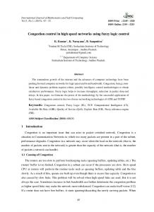
considered, and a compensator is developed to reduce the difference between the fuzzy constrained predictive controller output and the actual nonlinear control output. It is assumed that the actuator of every car in the high speed train has identical dynamics attributes, and the actuator dynamics in this brief are considered for the following case: Δ𝛿𝑎𝑖 (𝑘) = 𝛿𝑢𝑖 (𝑘) , Δ𝛿𝑢𝑖 (𝑘) = −𝑎𝛿𝑢𝑖 (𝑘) + 𝑏 (𝑢𝑖 (𝑘) − 𝛿𝑎𝑖 (𝑘)) ,
𝑢𝑐𝑖 (𝑘) =
𝑎, 𝑏 > 0,
where 𝑢𝑖 (𝑘) is control input of the 𝑖th car from the fuzzy predictive controller, 𝛿𝑎𝑖 (𝑘) is the actual control output imposed on the 𝑖th car, and 𝛿𝑢𝑖 (𝑘) is a virtual input. The overall structure of the compensation scheme consists of fuzzy predictive controller, actuator compensator, and actuator as depicted in Figure 2, where 𝑢𝑐 (𝑘) is the control input from actuator compensator. Next, based on Theorem 3, we will state our main results on the actuator compensator design for the fuzzy constrained predictive controller based on backstepping [36] approach. Theorem 5. Consider the actuator dynamics of high speed train as described by (43). If the 𝑖th control input 𝑢𝑐𝑖 (𝑘) from actuator compensator in Figure 2 is adjusted according to the equation
(43)
(𝑎𝛿𝑢𝑖 (𝑘) + 𝑏𝛿𝑎𝑖 (𝑘) + Δ2 𝑢𝑖 (𝑘) − 𝑘0 𝛿𝑢𝑖 (𝑘) + 𝑘0 Δ𝑢𝑖 (𝑘) − 𝑘0 𝑒2𝑖 (𝑘)) 𝑏
then it is ensured that the actual output of high speed train actuator asymptotically tracks the desired one given by the fuzzy constrained predictive controller in Theorem 3. Proof. Consider the control-loop system as shown in Figure 2. 𝑢𝑖 (𝑘) in the actuator dynamics (43) is changed into 𝑢𝑐𝑖 (𝑘) as Δ𝛿𝑎𝑖 (𝑘) = 𝛿𝑢𝑖 (𝑘) , Δ𝛿𝑢𝑖 (𝑘) = −𝑎𝛿𝑢𝑖 (𝑘) + 𝑏 (𝑢𝑐𝑖 (𝑘) − 𝛿𝑎𝑖 (𝑘)) , 𝑎, 𝑏 > 0,
(45)
(46)
Taking forward difference, we have Δ𝑒1𝑖 (𝑘) = Δ𝛿𝑎𝑖 (𝑘) − Δ𝑢𝑖 (𝑘) = 𝛿𝑢𝑖 (𝑘) − Δ𝑢𝑖 (𝑘) .
(47)
To apply the backstepping recursive design procedure, we start with the definition of the virtual input 𝛿𝑢𝑖 (𝑘) = Δ𝑢𝑖 (𝑘) − 𝑘0 𝑒1𝑖 (𝑘), where 𝑘0 is a constant. Then, one can obtain that Δ𝑒1𝑖 (𝑘) = −𝑘0 𝑒1𝑖 (𝑘) .
(48)
Proceeding to apply backstepping process, we introduce the following variable: 𝑒2𝑖 (𝑘) = 𝛿𝑢𝑖 (𝑘) − Δ𝑢𝑖 (𝑘) + 𝑘0 𝑒1𝑖 (𝑘) .
(44)
Taking forward difference, the above equation becomes Δ𝑒2𝑖 (𝑘) = Δ𝛿𝑢𝑖 (𝑘) − Δ2 𝑢𝑖 (𝑘) + 𝑘0 Δ𝑒1𝑖 (𝑘) = −𝑎𝛿𝑢𝑖 (𝑘) + 𝑏𝑢𝑐𝑖 (𝑘) − 𝑏𝛿𝑎𝑖 (𝑘) − Δ2 𝑢𝑖 (𝑘)
(50)
+ 𝑘0 𝛿𝑢𝑖 (𝑘) − 𝑘0 Δ𝑢𝑖 (𝑘) . Next, we construct the Lyapunov function candidate
where 𝑢𝑐𝑖 (𝑘) is the 𝑖th control input from the actuator compensator. For the purpose of maintaining the desired performance of the fuzzy constrained predictive controller, we should guarantee that 𝛿𝑎𝑖 (𝑘) will closely track 𝑢𝑖 (𝑘). Thus, the error is defined as 𝑒1𝑖 (𝑘) = 𝛿𝑎𝑖 (𝑘) − 𝑢𝑖 (𝑘) .
,
(49)
𝑉 (𝑘) = 𝑒12𝑖 (𝑘) + 𝑒22𝑖 (𝑘)
(51)
and also take its forward difference to obtain 𝑉 (𝑘 + 1) − 𝑉 (𝑘) = 𝑒12𝑖 (𝑘 + 1) + 𝑒22𝑖 (𝑘 + 1) − 𝑒12𝑖 (𝑘) − 𝑒22𝑖 (𝑘) = (2𝑒1𝑖 (𝑘) + Δ𝑒1𝑖 (𝑘)) Δ𝑒1𝑖 (𝑘)
(52)
+ (2𝑒2𝑖 (𝑘) + Δ𝑒2𝑖 (𝑘)) Δ𝑒2𝑖 (𝑘) . By combining (44), (48), and (50), we can obtain that condition (52) is equivalent to 𝑉 (𝑘 + 1) − 𝑉 (𝑘) = 𝑘0 (𝑘0 − 2) (𝑒12𝑖 (𝑘) + 𝑒22𝑖 (𝑘)) ,
(53)
which shows that the origin (𝑒1𝑖 = 0, 𝑒2𝑖 = 0) is asymptotically stable by appropriately choosing 𝑘0 . Therefore, the 𝑖th control input 𝑢𝑐𝑖 (𝑘) from actuator compensator in form of (44) is obtained to guarantee that the second-order actuator dynamics are reduced. This completes the proof. Remark 6. Theorem 5 develops a compensator using the backstepping technique to inhibit second-order actuator
Discrete Dynamics in Nature and Society
9
Table 1: The simulation parameters of high speed train. Value 80 × 103 0.06 80 × 103 0.01176 7.7616 × 10⁻⁴ 1.6 × 10⁻⁵
Unit kg — Nm−1 Nkg−1 Ns(mkg)−1 Ns2 (m2 kg)−1
dynamics for high speed train. It should be pointed out that the actuator dynamics associated with the control problem of high speed train are closely related to traction and braking actions. In practical operation, traction and braking actions are usually taken interchangeably by the control system. For the sake of simplicity, this paper addresses the train dynamic model during traction and braking phase in a unified form with different parameters, which can be achieved by tuning 𝑎 and 𝑏 in (43).
4. Numerical Simulations In this section, we will give numerical experiments to illustrate the effectiveness of the proposed method for the optimal control of high speed train. In these examples, we consider a high speed train with eight cars. The parameters of the high speed train are listed in Table 1, which are derived from the experimental results of the Japanese Shinkansen high speed train [17]. With the consideration of both theoretical and practical factors, the membership functions for the speed tracking error are chosen as shown in Figure 3. According to the above membership functions, the closeloop system of high speed train (17) can be transformed to 5
5
𝑥 (𝑘 + 1) = ∑ ∑ ℎ𝑙 (̂V1 (𝑘)) ℎ𝑚 (̂V1 (𝑘)) 𝑙=1 𝑚=1
⋅ [𝐴 𝑙 𝑥 (𝑘) + 𝐵𝑙 𝐹𝑚 𝑥 (𝑘)] , where −̂V (𝑘) − 20 { 1 , −40 ≤ ̂V1 (𝑘) < −20, ℎ1 (̂V1 (𝑘)) = { 20 ̂V1 (𝑘) < −40, {1, ℎ2 (̂V1 (𝑘)) ̂V (𝑘) + 20 + 20 { { 1 , −40 ≤ ̂V1 (𝑘) < 0, ={ 20 { 0, otherwise, { ̂V (𝑘) + 20 { { 1 , −20 ≤ ̂V1 (𝑘) < 20, ℎ3 (̂V1 (𝑘)) = { 20 { 0, otherwise, {
(54)
Degree of membership
1
Parameters Mass 𝑚𝑖 Rotary mass coefficient 𝑘 𝑐0 𝑐1 𝑐2
NB
NS
ZO
PS
PB
0.8 0.6 0.4 0.2 0 −50 −40 −30 −20 −10 0 10 Speed track error
20
30
40
50
Figure 3: The membership functions for the speed tracking error.
ℎ4 (̂V1 (𝑘)) ̂V (𝑘) − 20 + 20 { { 1 , 0 ≤ ̂V1 (𝑘) < −40, ={ 20 { 0, otherwise, { ̂V (𝑘) − 20 { 1 , 20 ≤ ̂V1 (𝑘) < 40, ℎ5 (̂V1 (𝑘)) = { 20 40 ≤ ̂V1 (𝑘) . {1, (55) In addition, 𝐴 𝑖 , 𝐵𝑖 , 𝑖 = 1, 2, . . . , 5, can be easily determined with respect to (11) and (54), which are not mentioned here to keep the paper concise. 4.1. Example 1. Regarding the parameters used in the controller design, the sampling period 𝑇𝑠 is 0.5 s, and the weights are 𝛼𝑓 = 4 × 10⁻⁷ , 𝛼𝑢 = 200, and 𝛼V = 0.5. For the optimal control of high speed train, the constraints for control input are determined not only by the physical characteristics of actuators but also by safety and comfort requirements. In practical optimal operations, the realistic constraint is usually far below the theoretical value of maximum traction effort. As a result, we adopt a usual and simplified constraint |𝑢𝑖 (𝑘)| ≤ 5 for the magnitude of control input in this research. Suppose that the high speed train is cruising at an initial speed V𝑖 = 180 km/h, 𝑖 = 1, . . . , 8, and the initial relative displacement between the two neighbouring cars is 𝑥𝑖 = 0, 𝑖 = 1, . . . , 8. The desired speed of the high speed train is given as follows: 180 km/h, { { { { V = {200 km/h, { { { {170 km/h, ∗
0 s ≤ 𝑡 < 100 s, 100 s ≤ 𝑡 < 1000 s,
(56)
1000 s ≤ 𝑡 ≤ 2000 s.
When actuator dynamics are not considered for high speed train, by applying the fuzzy constrained predictive control in Theorem 3, the fuzzy predictive control gain can
Discrete Dynamics in Nature and Society 210 200 190 180 170 160
0 100 200 300 400 500 600 700 800 900 1000 1100 1200 1300 1400 1500 1600 1700 1800 1900 2000
Speed (km/h)
10
Time (s)
1400
1600
1800
2000
1400
1600
1800
2000
1200
1000
800
600
400
200
0.1 0.05 0 −0.05 −0.1 0
Relative displacement (m)
(a)
Time (s)
1200
1000
800
600
400
200
0.2 0.1 0 −0.1 −0.2
0
Traction effort (kN/kg)
(b)
Time (s) (c)
Figure 4: Optimal curves for each car under the fuzzy constrained predictive controller.
be obtained as 𝐹𝑙 (𝑘) = 𝑌𝑙 (𝑘)𝐺(𝑘)−1 . With help of Matlab LMI toolbox, gain 𝐹𝑙 is solved efficiently and the minimum performance value is 𝛾∗ = 161588.5. As the dimensions for gain 𝐹𝑙 are very large, it is not given here to keep the paper concise. Under the fuzzy constrained predictive control, the running speed curves for each high speed train are plotted in Figure 4(a), where the velocity curves for each car are described in solid line and the dotted line denotes the desired speed. It shows that, at the initial time, each car of the high speed train tracks the desired speed V∗ = 180 km/h. Then, at the time 𝑡 = 100 s, the desired speed for high speed train increases to 200 km/h, and each car of high speed train begins to accelerate to track the reference speed. We can find out that each car of high speed train can perfectly track the desired speed V∗ = 200 km/h after 𝑡 = 432 s and the acceleration phrase lasts nearly 332 seconds. From 𝑡 = 1000 s, the reference speed changes to 170 km/h, and each car of high speed train begins to brake to track the predefined speed. We can observe that the speeds of each car are eventually kept at the equilibrium state (zero point) from 1428 s. It is easy to calculate that the mean acceleration rate is approximately 0.06 m/s2 , which ensures the safety and comfort of the operation of the high speed train. It can be inferred from the above results that although maximum traction force is usually adopted in an energy-efficient driving strategy, it may not be the optimal choice when other factors such as speed tracking and in-train forces are contemplated as a whole. The evolution curves of relative coupler displacements between two neighboring cars are shown in Figure 4(b). When the high speed train starts to accelerate or decelerate,
the deviations of the relative coupler displacements go up remarkably at the beginning of acceleration or deceleration phrase. As the speed is approaching the desired one, the absolute values of the displacements follow a downward trend. In the end, the relative coupler displacements between the two connected cars are stabilized at the equilibrium state (zero point). It is obvious that the deviations of the relative coupler displacements from the equilibrium state remain positive in the acceleration phase (i.e., generating traction force in the longitudinal direction) and become negative when the train begins to decelerate (i.e., generating braking force in the longitudinal direction), which are in accordance with practice. Meanwhile, the deviations of relative spring displacements for each car are effectively controlled in the reasonable range of 0.07 m during the whole journey, which ensure the safety and comfort of the operation of the high speed train. Correspondingly, the control forces 𝑢𝑖 (𝑘) for each train are plotted in Figure 4(c), which show that at the beginning the control forces 𝑢𝑖 (𝑘) for each train are very big for tracking the desired speed, and when the tracking goal of the fuzzy constrained predictive control is achieved, the control forces are reduced and converge to a constant. From what has been discussed above, it can be concluded that the fuzzy constrained predictive design approach is able to schedule the train to track the reference speed profile without violating any operational constraints. 4.2. Example 2. Then, under the case of actuator dynamics, we will consider the fuzzy constrained predictive control of high speed train. The actuator model is chosen as (43) with 𝑎 = 14 and 𝑏 = 100 during traction phase and with 𝑎 = 20 and 𝑏 = 150 for braking phase. Other control parameters remain the same as in Example 1 and the simulation results are given in Figure 5. By comparing to Figure 4, it is shown that, at the beginning of the acceleration and deceleration periods, the speed, relative coupler displacements between the two connected cars, and control forces with actuator dynamics have bigger fluctuations than the case without actuator dynamics. These unstable behaviors may be quite uncomfortable for passengers. In addition, all the speeds of each car with actuator dynamics track the desired speed slower than the case without actuator dynamics. The acceleration phrase undergoes nearly 480 s and the deceleration phrase lasts almost 620 s compared to 332 s and 432 s in Example 1, respectively, which clearly indicate that the actuator dynamics will lead to the degradation of the fuzzy constrained predictive controller. We further consider the case where the actuator compensator in Figure 2 is introduced to counterbalance the effect of actuator dynamics. According to Theorem 5, by applying 𝑢𝑐𝑖 (𝑘) to each car, the running curves are depicted in Figure 6. From Figure 6, we can observe that, in the beginning, due to the big gap with the desired speed, all the cars are running with the traction forces. After 𝑡 = 1000 s, each car of high speed train begins to brake to track the lower reference speed. It can be clearly found that the fluctuations in Figure 5 are effectively handled, and both the relative spring displacements and speed of each car are finally kept
210 200 190 180 170 160
210 200 190 180 170 160
0 100 200 300 400 500 600 700 800 900 1000 1100 1200 1300 1400 1500 1600 1700 1800 1900 2000
Speed (km/h)
11
0 100 200 300 400 500 600 700 800 900 1000 1100 1200 1300 1400 1500 1600 1700 1800 1900 2000 Time (s)
Time (s)
Time (s)
1400
1600
1800
2000
1600
1800
2000
1200
1000
800
600
400
200
0.2 0.1 0 −0.1 −0.2
0
Traction effort (kN/kg)
2000
1800
1600
1400
1200
(b)
1000
800
600
400
200
0
Traction effort (kN/kg)
1200
Time (s)
(b)
0.2 0.1 0 −0.1 −0.2
1400
Time (s)
1000
600
400
200
0.1 0.05 0 −0.05 −0.1 0
2000
1800
1600
1400
1200
1000
800
600
400
200
Relative displacement (m)
(a)
0.1 0.05 0 −0.05 −0.1 0
Relative displacement (m)
(a)
800
Speed (km/h)
Discrete Dynamics in Nature and Society
Time (s)
(c)
(c)
Figure 5: Optimal curves for each car under the fuzzy constrained predictive controller with actuator dynamics.
Figure 6: Optimal curves for each car under the fuzzy constrained predictive controller with actuator compensator.
at the equilibrium state (zero point), which indicates the effectiveness of the proposed actuator compensator scheme. To better show the effectiveness of the proposed actuator compensation method, we give some sensitivity analysis under different conditions. Then the case without actuator dynamics (Case 1), the case with actuator dynamics (Case 2), and the case with actuator compensator (Case 3) are plotted in Figure 7. For the convenience of comparing, we calculate the mean values of speeds, relative spring displacements, and forces for the three cases. From these simulation results, it can be seen that, during the whole travel, the mean speed curve and mean traction effort in Case 3 can exactly track the ideal results in Case 1, which also takes shorter time to reach the equilibrium state than Case 2. Moreover, the max value of mean relative spring displacements is much smaller due to the actuator compensator, which greatly enhances safety for high speed train movement. In addition, simulations are carried out to investigate the effects of 𝛼𝑓 , 𝛼𝑢 , and 𝛼V on the train’s performance, which allow the proposed controller to make some adjustments with in-train force minimization, energy consumption reduction, and velocity tracking improvement. In order to facilitate energy consumption analysis in different control strategies, 𝑇 we use 𝐸 = ∫𝑡 𝑓 |𝑢𝑖 V𝑖 |𝑑𝑡 to approximate the energy consumed 0 during the optimizing interval. Under the fuzzy constrained predictive controller with actuator compensator, the energy consumption, duration time, and max coupler displacement during the acceleration phase are summarized in Table 2. First, we augment 𝛼𝑢 from 200 to 2000 and the other two parameters remain the same as in Example 1, which implies
that controller is tuned to be an energy efficiency-emphasized one. Consequently, energy consumption decreases from 29856 MJ to 29678 MJ. By contrast, the acceleration time is longer and the max coupler displacement is larger compared to the case in Example 1, which results in worse speed tracking results, and in-train forces increase. To examine what exactly happens when attention is paid on better velocity tracking results, we change 𝛼V from 0.5 to 10, and the other parameters are the same as those presented in the above example unless otherwise noted. We can observe that it takes as soon as 314 s to catch the desired speed with 𝛼V = 10 compared to 360 s with 𝛼V = 0.5. This phenomenon can be explained by the reason that more efforts are exerted on each car to prompt the velocity in a shorter time, thereby leading to the fact that the maximum traction effort and energy consumption have a slight rise in this case. Thus, the emphasized performance would be better, while the other two aspects of the performance would deteriorate. In practice, we should coordinate the three parameters with regard to the desired performance.
5. Conclusion In this brief, we investigate the problem of fuzzy predictive cruise control of high speed train such that the objective function value of train performance criteria is optimized at every step in infinite time horizon subject to input constraints. Employing Takagi-Sugeno (T-S) fuzzy model, we approximate the high speed train system to an interpolation of some local linear models by fuzzy membership functions. Based on Lyapunov stability theory, a set of LMIs is given
Discrete Dynamics in Nature and Society
200
200
Speed (km/h)
Speed (km/h)
12
190 180 170
100 150 200 250 300 350 400 450 500 550 600 Time (s)
190 180 170 1000
1100
1200
1500
1600
(b)
0.04 0.03 0.02 0.01 0 100 150 200 250 300 350 400 450 500 550 600 Time (s)
Relative displacement (m)
Relative displacement (m)
(a)
0 −0.02 −0.04 −0.06 1000
Case 1 Case 2 Case 3
1100
1200
1300 Time (s)
1400
1500
1600
Case 1 Case 2 Case 3 (c)
(d)
0.2
Traction effort (kN/kg)
Traction effort (kN/kg)
1400
Case 1 Case 2 Case 3
Case 1 Case 2 Case 3
−0.01
1300 Time (s)
0.15 0.1 0.05 0 100 150 200 250 300 350 400 450 500 550 600 Time (s) Case 1 Case 2 Case 3
0 −0.05 −0.1 −0.15 −0.2 1000
1100
1200
1300 Time (s)
1400
1500
1600
Case 1 Case 2 Case 3 (e)
(f)
Figure 7: Simulation results with different control weights.
Table 2: The simulation results with different control weights. Item Energy consumption (MJ) Acceleration time (s) Max coupler displacement (m)
𝛼𝑓 = 4 × 10⁻⁷ , 𝛼𝑢 = 200 𝛼V = 0.5 29856 332 0.0544
to solve the corresponding controller optimization problem which guarantees the various railway operational performances such as safety, energy consumption, riding comfort, and velocity tracking. Moreover, a mathematically rigorous and algorithmically tractable actuator compensator is added to adjust the output of the fuzzy constrained predictive
𝛼𝑓 = 4 × 10⁻⁷ , 𝛼𝑢 = 2000 𝛼V = 0.5 29678 360 0.0578
𝛼𝑓 = 4 × 10⁻⁷ , 𝛼𝑢 = 2000 𝛼V = 10 29947 314 0.0592
controller in the presence of traction and braking dynamics, which greatly enhances safety and comfort for high speed train movement. The effectiveness and applicability of the proposed method are further examined through numerical experiments. Additionally, we notice that if the number of cars increases, the computational time in the proposed
Discrete Dynamics in Nature and Society algorithm may increase drastically. Then, one may resort to the distributed MPC design method, which needs to be investigated in the future.
Competing Interests The authors declare that they have no competing interests.
Acknowledgments This paper was partially supported by Beijing Laboratory of Urban Rail Transit and Beijing Key Laboratory of Urban Rail Transit Automation and Control, by Beijing Jiaotong University Technology Funding Project under Grant 2016JBM005, by the Foundation for the Author of the National Excellent Doctoral Dissertation of China under Grant 201449, and by the National Natural Science Foundation under Grant 61573056.
References [1] H. R. Dong, B. Ning, B. G. Cai, and Z. S. Hou, “Automatic train control system development and simulation for highspeed railways,” IEEE Circuits and Systems Magazine, vol. 10, no. 2, pp. 6–18, 2010. [2] L. Li, W. Dong, Y. Ji, Z. Zhang, and L. Tong, “Minimal-energy driving strategy for high-speed electric train with hybrid system model,” IEEE Transactions on Intelligent Transportation Systems, vol. 14, no. 4, pp. 1642–1653, 2013. [3] X. Li, C.-F. Chien, L. Li, Z. Y. Gao, and L. Yang, “Energyconstraint operation strategy for high-speed railway,” International Journal of Innovative Computing, Information and Control, vol. 8, no. 10, pp. 6569–6583, 2013. [4] P. Howlett, “Optimal strategies for the control of a train,” Automatica, vol. 32, no. 4, pp. 519–532, 1996. [5] P. Howlett, “The optimal control of a train,” Annals of Operations Research, vol. 98, no. 1–4, pp. 65–87, 2000. [6] E. Khmelnitsky, “On an optimal control problem of train operation,” IEEE Transactions on Automatic Control, vol. 45, no. 7, pp. 1257–1266, 2000. [7] R. Chevrier, P. Pellegrini, and J. Rodriguez, “Energy saving in railway timetabling: a bi-objective evolutionary approach for computing alternative running times,” Transportation Research Part C: Emerging Technologies, vol. 37, pp. 20–41, 2013. [8] B.-R. Ke, C.-L. Lin, and C.-W. Lai, “Optimization of train-speed trajectory and control for mass rapid transit systems,” Control Engineering Practice, vol. 19, no. 7, pp. 675–687, 2011. [9] K. Kim and S. I.-J. Chien, “Optimal train operation for minimum energy consumption considering track alignment, speed limit, and schedule adherence,” Journal of Transportation Engineering, vol. 137, no. 9, pp. 665–674, 2011. [10] L. X. Yang, K. P. Li, Z. Y. Gao, and X. Li, “Optimizing trains movement on a railway network,” Omega, vol. 40, no. 5, pp. 619– 633, 2012. [11] R. Su, Q. Gu, and T. Wen, “Optimization of high-speed train control strategy for traction energy saving using an improved genetic algorithm,” Journal of Applied Mathematics, vol. 10, no. 2, pp. 1–7, 2014.
13 [12] P. Gruber and M. M. Bayoumi, “Suboptimal control strategies for multilocomotive powered trains,” IEEE Transactions on Automatic Control, vol. 27, no. 3, pp. 536–546, 1982. [13] X. Zhuan and X. Xia, “Cruise control scheduling of heavy haul trains,” IEEE Transactions on Control Systems Technology, vol. 14, no. 4, pp. 757–766, 2006. [14] X. Zhuan and X. Xia, “Optimal scheduling and control of heavy haul trains equipped with electronically controlled pneumatic braking systems,” IEEE Transactions on Control Systems Technology, vol. 15, no. 6, pp. 1159–1166, 2007. [15] Q. Song, Y.-D. Song, T. Tang, and B. Ning, “Computationally inexpensive tracking control of high-speed trains with traction/braking saturation,” IEEE Transactions on Intelligent Transportation Systems, vol. 12, no. 4, pp. 1116–1125, 2011. [16] S. K. Li, L. X. Yang, K. P. Li, and Z. Y. Gao, “Robust sampled-data cruise control scheduling of high speed train,” Transportation Research Part C: Emerging Technologies, vol. 46, pp. 274–283, 2014. [17] S.-K. Li, L.-X. Yang, and K.-P. Li, “Robust output feedback cruise control for high-speed train movement with uncertain parameters,” Chinese Physics B, vol. 24, no. 1, Article ID 010503, 2015. [18] L. Zhang and X. Zhuan, “Optimal operation of heavy-haul trains equipped with electronically controlled pneumatic brake systems using model predictive control methodology,” IEEE Transactions on Control Systems Technology, vol. 22, no. 1, pp. 13–22, 2014. [19] K. Tanaka and M. Sugeno, “Stability analysis and design of fuzzy control systems,” Fuzzy Sets and Systems, vol. 45, no. 2, pp. 135– 156, 1992. [20] G. Feng, “A survey on analysis and design of model-based fuzzy control systems,” IEEE Transactions on Fuzzy Systems, vol. 14, no. 5, pp. 676–697, 2006. [21] Y. Zhao, B. Li, J. H. Qin, H. J. Gao, and H. R. Karimi, “𝐻∞ consensus and synchronization of nonlinear systems based on a novel fuzzy model,” IEEE Transactions on Cybernetics, vol. 43, no. 6, pp. 2157–2169, 2013. [22] S. Yasunobu, S. Miyamoto, T. Takaoka, and H. Oshima, “Application of predictive fuzzy control to automatic train operation controller,” in Proceedings of the IEEE International Conference on Industrial Electronics, Control and Instrumentation, pp. 657– 662, 1984. [23] H.-R. Dong, S.-G. Gao, B. Ning, and L. Li, “Extended fuzzy logic controller for high speed train,” Neural Computing and Applications, vol. 22, no. 2, pp. 321–328, 2013. [24] C. Sicre, A. P. Cucala, and A. Fern´andez-Cardador, “Real time regulation of efficient driving of high speed trains based on a genetic algorithm and a fuzzy model of manual driving,” Engineering Applications of Artificial Intelligence, vol. 29, pp. 79– 92, 2014. [25] C. D. Yang and Y. P. Sun, “Mixed h2 /h∞ cruise controller design for high speed train,” IEEE Transactions on Control Systems Technology, vol. 74, no. 9, pp. 905–920, 2001. [26] A. P. Cucala, A. Fern´andez, C. Sicre, and M. Dom´ınguez, “Fuzzy optimal schedule of high speed train operation to minimize energy consumption with uncertain delays and drivers behavioral response,” Engineering Applications of Artificial Intelligence, vol. 25, no. 8, pp. 1548–1557, 2012. [27] Y. Xia, G.-P. Liu, M. Fu, and D. Rees, “Predictive control of networked systems with random delay and data dropout,” IET Control Theory and Applications, vol. 3, no. 11, pp. 1476–1486, 2009.
14 [28] Y. Zhao, H. J. Gao, and T. Chen, “Fuzzy constrained predictive control of non-linear systems with packet dropouts,” IET Control Theory & Applications, vol. 4, no. 9, pp. 1665–1677, 2010. [29] Q. Song, Y. D. Song, and W. Cai, “Adaptive backstepping control of train systems with traction/braking dynamics and uncertain resistive forces,” Vehicle System Dynamics, vol. 49, no. 9, pp. 1441–1454, 2011. [30] M. Krstic, I. Kanellakopoulos, and P. Kokotovic, Nonlinear and Adaptive Control Design, Wiley, New York, NY, USA, 1995. [31] M. Chou and X. Xia, “Optimal cruise control of heavy-haul trains equipped with electronically controlled pneumatic brake systems,” Control Engineering Practice, vol. 15, no. 5, pp. 511–519, 2007. [32] W. J. Davis, “The tractive resistance of electric locomotives and cars,” General Electric Review, vol. 29, no. 10, pp. 685–707, 1926. [33] K. Tanaka and H. O. Wang, Fuzzy Control Systems Design and Analysis: A Linear Matrix Inequality Approach, John Wiley & Sons, New York, NY, USA, 2001. [34] F. A. Cuzzola, J. C. Geromel, and M. Morari, “An improved approach for constrained robust model predictive control,” Automatica, vol. 38, no. 7, pp. 1183–1189, 2002. [35] X.-P. Guan and C.-L. Chen, “Delay-dependent guaranteed cost control for T-S fuzzy systems with time delays,” IEEE Transactions on Fuzzy Systems, vol. 12, no. 2, pp. 236–249, 2004. [36] H. K. Khalil and J. W. Grizzle, Nonlinear Systems, Prentice Hall, Upper Saddle River, NJ, USA, 1996.
Discrete Dynamics in Nature and Society
Advances in
Operations Research Hindawi Publishing Corporation http://www.hindawi.com
Volume 2014
Advances in
Decision Sciences Hindawi Publishing Corporation http://www.hindawi.com
Volume 2014
Journal of
Applied Mathematics
Algebra
Hindawi Publishing Corporation http://www.hindawi.com
Hindawi Publishing Corporation http://www.hindawi.com
Volume 2014
Journal of
Probability and Statistics Volume 2014
The Scientific World Journal Hindawi Publishing Corporation http://www.hindawi.com
Hindawi Publishing Corporation http://www.hindawi.com
Volume 2014
International Journal of
Differential Equations Hindawi Publishing Corporation http://www.hindawi.com
Volume 2014
Volume 2014
Submit your manuscripts at http://www.hindawi.com International Journal of
Advances in
Combinatorics Hindawi Publishing Corporation http://www.hindawi.com
Mathematical Physics Hindawi Publishing Corporation http://www.hindawi.com
Volume 2014
Journal of
Complex Analysis Hindawi Publishing Corporation http://www.hindawi.com
Volume 2014
International Journal of Mathematics and Mathematical Sciences
Mathematical Problems in Engineering
Journal of
Mathematics Hindawi Publishing Corporation http://www.hindawi.com
Volume 2014
Hindawi Publishing Corporation http://www.hindawi.com
Volume 2014
Volume 2014
Hindawi Publishing Corporation http://www.hindawi.com
Volume 2014
Discrete Mathematics
Journal of
Volume 2014
Hindawi Publishing Corporation http://www.hindawi.com
Discrete Dynamics in Nature and Society
Journal of
Function Spaces Hindawi Publishing Corporation http://www.hindawi.com
Abstract and Applied Analysis
Volume 2014
Hindawi Publishing Corporation http://www.hindawi.com
Volume 2014
Hindawi Publishing Corporation http://www.hindawi.com
Volume 2014
International Journal of
Journal of
Stochastic Analysis
Optimization
Hindawi Publishing Corporation http://www.hindawi.com
Hindawi Publishing Corporation http://www.hindawi.com
Volume 2014
Volume 2014