Winner-Takes-All algorithms, on-line learning, competitive learning. 1 Introduction. Learning ..... [14] S. Seo, M. Bode, and K. Obermayer. Soft nearest prototype ...
Learning Vector Quantization: The Dynamics of Winner-Takes-All Algorithms Michael Biehl1 , Anarta Ghosh1 , and Barbara Hammer2 1- Rijksuniversiteit Groningen - Mathematics and Computing Science P.O. Box 800, NL-9700 AV Groningen - The Netherlands 2- Clausthal University of Technology - Institute of Computer Science D-98678 Clausthal-Zellerfeld - Germany Abstract Winner-Takes-All (WTA) prescriptions for Learning Vector Quantization (LVQ) are studied in the framework of a model situation: Two competing prototype vectors are updated according to a sequence of example data drawn from a mixture of Gaussians. The theory of on-line learning allows for an exact mathematical description of the training dynamics, even if an underlying cost function cannot be identified. We compare the typical behavior of several WTA schemes including basic LVQ and unsupervised Vector Quantization. The focus is on the learning curves, i.e. the achievable generalization ability as a function of the number of training examples.
Keywords: Learning Vector Quantization, prototype-based classification, Winner-Takes-All algorithms, on-line learning, competitive learning
1
Introduction
Learning Vector Quantization (LVQ) as originally proposed by Kohonen [10] is a widely used approach to classification. It is applied in a variety of practical problems, including medical image and data analysis, e.g. proteomics, classification of satellite spectral data, fault detection in technical processes, and language recognition, to name only a few. An overview and further references can be obtained from [1]. LVQ procedures are easy to implement and intuitively clear. The classification of data is based on a comparison with a number of so-called prototype vectors. The similarity is frequently measured in terms of Euclidean 1
distance in feature space. Prototypes are determined in a training phase from labeled examples and can be interpreted in a straightforward way as they directly represent typical data in the same space. This is in contrast with, say, adaptive weights in feedforward neural networks or support vector machines which do not allow for immediate interpretation as easily. Among the most attractive features of LVQ is the natural way in which it can be applied to multi-class problems. In the simplest so-called hard or crisp schemes any feature vector is assigned to the closest of all prototypes and the corresponding class. In general, several prototypes will be used to represent each class. Extensions of the deterministic assignment to a probabilistic soft classification are conceptually straightforward but will not be considered here. Plausible training prescriptions exist which employ the concept of on-line competitive learning: Prototypes are updated according to their distance from a given example in a sequence of training data. Schemes in which only the winner, i.e. the currently closest prototype is updated have been termed Winner-Takes-All algorithms and we will concentrate on this class of prescriptions here. The ultimate goal of the training process is, of course, to find a classifier which labels novel data correctly with high probability, after training. This so-called generalization ability will be in the focus of our analysis in the following. Several modifications and potential improvements of Kohonen’s original LVQ procedure have been suggested. They aim at achieving better approximations of Bayes optimal decision boundaries, faster or more robust convergence, or the incorporation of more flexible metrics, to name a few examples [5, 8–10, 16]. Many of the suggested algorithms are based on plausible but purely heuristic arguments and they often lack a thorough theoretical understanding. Other procedures can be derived from an underlying cost function, such as Generalized Relevance LVQ [8,9] or LVQ2.1, the latter being a limit case of a statistical model [14, 15]. However, the connection of the cost functions with the ultimate goal of training, i.e. the generalization ability, is often unclear. Furthermore, several learning rules display instabilities and divergent behavior and require modifications such as the window rule for LVQ2.1 [10]. Clearly, a better theoretical understanding of the training algorithms should be helpful in improving their performance and in designing novel, more efficient schemes. In this work we employ a theoretical framework which makes possible a systematic investigation and comparison of LVQ training procedures. We 2
consider on-line training from a sequence of uncorrelated, random training data which is generated according to a model distribution. Its purpose is to define a non-trivial structure of data and facilitate our analytical approach. We would like to point out, however, that the training algorithms do not make use of the form of this distribution as, for instance, density estimation schemes. The dynamics of training is studied by applying the successful theory of online learning [3, 6, 12] which relates to ideas and concepts known from Statistical Physics. The essential ingredients of the approach are (1) the consideration of high-dimensional data and large systems in the so-called thermodynamic limit and (2) the evaluation of averages over the randomness or disorder contained in the sequence of examples. The typical properties of large systems are fully described by only a few characteristic quantities. Under simplifying assumptions, the evolution of these so-called order parameters is given by deterministic coupled ordinary differential equations (ODE) which describe the dynamics of on-line learning exactly in the thermodynamic limit. For reviews of this very successful approach to the investigation of machine learning processes consult, for instance, [3, 6, 17]. The formalism enables us to compare the dynamics and generalization ability of different WTA schemes including basic LVQ1 and unsupervised Vector Quantization (VQ). The analysis can readily be extended to more general schemes, approaching the ultimate goal of designing novel and efficient LVQ training algorithms with precise mathematical foundations. The paper is organized as follows: in the next section we introduce the model, i.e. the specific learning scenarios and the assumed statistical properties of the training data. The mathematical description of the training dynamics is briefly summarized in section 3, technical details are given in an appendix. Results concerning the WTA schemes are presented and discussed in section 4 and we conclude with a summary and an outlook on forthcoming projects.
2 2.1
The model Winner-Takes-All algorithms
We study situations in which input vectors ξ ∈ IR N belong to one of two possible classes denoted as σ = ±1. Here, we restrict ourselves to the case of two prototype vectors wS where the label S = ±1 (or ± for short) corresponds to the represented class.
3
In all WTA-schemes, the squared Euclidean distances d S (ξ) = (ξ − wS )2 are evaluated for S = ±1 and the vector ξ is assigned to class σ if d +σ < d−σ . We investigate incremental learning schemes in which a sequence of single, uncorrelated examples {ξ µ , σ µ } is presented to the system. The analysis can be applied to a larger variety of algorithms but here we treat only updates of the form � � η µ ΘS g(S, σ µ ) ξ µ − w Sµ−1 . (1) wµS = wSµ−1 + ∆wµS with ∆wµS = N Here, the vector w µS denotes the prototype after presentation of µ examples and the learning rate η is rescaled with the vector dimension N . The Heaviside term � 1 if x > 0. µ µ µ ΘS = Θ(d−S − d+S ) with Θ(x) = 0 else
singles out the current prototype w Sµ−1 which is closest to the new input ξ µ in the sense of the measure dµS = (ξ µ − wSµ−1 )2 . In this formulation, only the winner, say, w S can be updated whereas the looser w −S remains unchanged. The change of the winner is always along the direction ±(ξ µ − wµ−1 S ). The function g(S, σ µ ) further specifies the update rule. Here, we focus on three special cases of WTA learning: I) LVQ1: g(S, σ) = Sσ = +1 (resp. − 1) for S = σ (resp. S 6= σ). This extension of competitive learning to labeled data corresponds to Kohonen’s original LVQ1. The update is towards ξ µ if the example belongs to the class represented by the winning prototype, the correct winner. On the contrary, a wrong winner is moved away from the current input. II) LVQ+: g(S, σ) = Θ(Sσ) = +1 (resp. 0) for S = σ (resp. S 6= σ). In this scheme the update is non-zero only for a correct winner and, then, always positive. Hence, a prototype w S can only accumulate updates from its own class σ = S. We will use the abbreviation LVQ+ for this prescription. III) VQ: g(S, σ) = 1. This update rule disregards the actual data label and always moves the winner towards the example input. It corresponds to unsupervised Vector Quantization and aims at finding prototypes which yield a good representation of the data in the sense of Euclidean distances. The choice g(S, σ) = 1 can also be interpreted as describing two prototypes which represent the same class and compete for updates from examples of this very class, only. 4
h−
b−
h+
b+
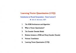
Figure 1: Data as generated according to the model density (3) in N = 200 dimension with p− = 0.6, p+ = 0.4. Open (filled) circles represent 240 (160) vectors ξ from clusters centered about orthonormal vectors `B + (`B − ) with ` = 1.5. The left panel shows the projections h ± = w± · ξ of the data on a randomly chosen pair of orthogonal unit vectors w ± , whereas the right panel displays b± = B · ξ, i.e. the plane spanned by B + , B − ; crosses mark the position of the cluster centers. Note that the VQ procedure (III) can be readily formulated as a stochastic gradient descent with respect to the quantization error e(ξ µ ) =
X 1 (ξ µ − w Sµ−1 )2 Θ(dµ−S − dµ+S ), 2
(2)
S=±1
see e.g. [7] for details. While intuitively clear and well motivated, LVQ1 (I) and LVQ+ (II) lack such a straightforward interpretation and relation to a cost function.
2.2
The model data
In order to analyse the behavior of the above algorithms we assume that randomized data is generated according to a model distribution P (ξ). As a simple yet non-trivial situation we consider input data drawn from a binary mixture of Gaussian clusters � � X 1 1 2 P (ξ) = pσ P (ξ | σ) with P (ξ | σ) = √ N exp − (ξ − λB σ ) 2 2π σ=±1 (3) 5
where the weights pσ correspond to the prior class membership probabilities and p+ + p− = 1. Clusters are centered about λB + and λB − , respectively. We assume that B σ · B τ = Θ(στ ), i.e. B 2σ = 1 and B + · B − = 0. The latter condition fixes the location of the cluster centers with respect to the origin while the parameter λ controls their separation. We consider the case where the cluster membership σ coincides with the class label of the data. The corresponding classification scheme is not linearly separable because the Gaussian contributions P (ξ |σ) overlap. According to Eq. (3) a vector ξ consists of statistically independent components with unit variance. Denoting the average over P (ξ | σ) by h· · · i σ we have, for instance, hξj iσ = λ(B σ )j for a component and correspondingly N � N � X X
2�
2� 1 + hξj i2σ = N + λ2 . ξj σ = ξ σ= j=1
j=1
P Averages over the full P (ξ) will be written as h· · · i = σ=±1 h· · · iσ . Note that in high dimensions, i.e. for large N , the Gaussians overlap significantly. The cluster structure of the data becomes only apparent when projected into the plane spanned by {B + , B − }. However projections in a randomly chosen two-dimensional subspace would overlap completely. Figure 1 illustrates the situation for Monte Carlo data in N = 200 dimensions. In an attempt to learn the classification scheme, the relevant directions B ± ∈ IRN have to be identified to a certain extent. Obviously this task becomes highly non-trivial for large N .
3
The dynamics of learning
The following analysis is along the lines of on-line learning, see e.g. [3,6,12]. for a comprehensive overview and example applications. In this section we briefly outline the treatment of WTA algorithms in LVQ and refer to appendix A for technical details. The actual configuration of prototypes is characterized by the projections µ RSσ = wµS · B σ
and QµST = wµS · wµT ,
for S, T, σ = ±1
(4)
The self-overlaps Q++ and Q−− specify the lengths of vectors w ± , whereas the remaining five overlaps correspond to projections, i.e. angles between w+ and w− and between the prototypes and the center vectors B ± .
6
The algorithm (1) directly implies recursions for the above defined quantities upon presentation of a novel example: � � µ µ−1 µ−1 N (RSσ − RSσ ) = η ΘµS g(S, σ µ ) bµS − RSσ � � µ−1 µ−1 ) = η ΘµS g(S, σ µ ) hµT − QST N (QµST − QST � � µ−1 + η ΘµT g(T, σ µ ) hµS − QST + η 2 ΘµS ΘµT g(S, σ µ ) g(T, σ µ ) + O(1/N )
(5)
Here, the actual input ξ µ enters only through the projections hµS = wSµ−1 · ξ µ
and bµσ = B σ · ξ µ .
(6)
µ−1 µ−1 Note in this context that ΘµS = Θ(Q−S−S − 2hµ−S − QSS + 2hµS ) also does not depend on ξ µ explicitly. An important assumption is that all examples in the training sequence are independently drawn from the model distribution and, hence, are uncorµ−1 related with previous data and with w ± . As a consequence, the statistics of the projections (6) are well known for large N . By means of the Central Limit Theorem their joint density becomes a mixture of Gaussians, which is fully specified by the corresponding conditional first and second moments:
� �
µ�
µ µ� µ−1 hS σ = λRSσ , hbµτ iσ = λΘ(τ σ), hS hT σ − hµS σ hµT σ = Qµ−1 ST
µ� µ
µ� µ
µ µ�
µ µ� µ−1 (7) bρ bτ σ − bρ σ hbτ iσ = Θ(ρτ ), hS bτ σ − hS σ hbτ iσ = RSτ ,
see the appendix for derivations. This observation enables us to perform an average of the recursions w.r.t. the latest example data in terms of Gaussian integrations. Details of the calculation are presented in appendix A, see also [4]. On the right hand sides of order (1/N ) have been
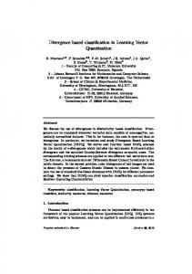
2 � of (5) terms 2 neglected using, for instance, ξ /N = 1 + λ /N ≈ 1 for large N . The limit N → ∞ has further simplifying consequences. First, the averaged recursions can be interpreted as ordinary differential equations (ODE) in continuous training time α = µ/N . Second, the overlaps {R Sσ , QST } as functions of α become self–averaging with respect to the random sequence of examples. Fluctuations of these quantities, as for instance observed in computer simulations of the learning process, vanish with increasing N and the description in terms of mean values is sufficient. For a detailed mathematical discussion of this property see [11]. Given initial conditions {RSσ (0), QST (0)}, the resulting system of coupled ODE can be integrated numerically. This yields the evolution of overlaps (4) with increasing α in the course of training. The behavior of the 7
2.0 1.0
R−−
6.0
R++
4.0
Q−− Q++
2.0 0.0 -1.0 50
100
150
200
250
R−+
0.0
R+−
-2.0 0
300
α
Q+− 50
100
150
200
250
300
α
Figure 2: The characteristic overlaps R Sσ (left panel) and QST (right panel) vs. the rescaled number of examples α = µ/N for LVQ1 with p + = 0.8, λ = 1, and η = 0.2. The solid lines display the result of integrating the system of ODE, symbols correspond to Monte Carlo simulations for N = 200 on average over 100 independent runs. Error bars are smaller than the symbol size. Prototypes were initialized close to the origin with R Sσ = Q+− = 0 and Q++ = Q−− = 10−4 . system will depend on the characteristics of the data, i.e. the separation λ, the learning rate η, and the actual algorithm as specified by the choice of g(S, σ) in Eq. (1). Monte Carlo simulations of the learning process are in excellent agreement with the N → ∞ theory for dimensions as low as N = 200 already, see Figure 2 for a comparison in the case of LVQ1. Our simulations furthermore confirm that the characteristic overlaps {R Sσ (α), QST (α)} are self-averaging quantities: their standard deviation determined from independent runs vanishes as N → ∞, details will be published elsewhere. The success of learning can be quantified as the probability of misclassiP fying novel random data, the generalization error � g = σ=±1 pσ hΘ−σ iσ . Performing the averages is done along the lines discussed above, see the appendix and [4]. One obtains �g as a function of the overlaps {QST , RSσ }: � � X QSS − Q−S−S − 2λ [RSS − R−SS ] √ , (8) �g = pσ Φ Q++ + Q−− − 2Q+− S=±1
Rx 2 where φ(x) = −∞ √dt2π e−t /2 . Hence, by inserting {QST (α), RSσ (α)} we can evaluate the learning curve �g (α), i.e. the typical generalization error as achieved from a sequence of αN examples.
8
�g
0.5
0.5
0.4
�g 0.4 0.3
0.3
0.2
0.2 0.1
0.1 100
α
0
200
0
0.5
p+
1
Figure 3: Left panel: Typical learning curves � g (α) of unsupervised VQ (dotted), LVQ+ (dashed) and LVQ1 (solid line) for λ = 1.0 and learning rate η = 0.2. Right panel: asymptotic �g for η → 0, ηα → ∞ for λ = 1.2 as a function of the prior weight p+ . The lowest, solid curve corresponds to the optimum �min whereas the dashed line represents the typical outcome of LVQ1. The g horizontal line is the p± –independent result for LVQ+, it can even exceed �g = min {p+ , p− } (thin solid line). Unsupervised VQ yields an asymptotic �g as marked by the chain line.
4 4.1
Results The dynamics
The dynamics of unsupervised VQ, setting III in section 2.1, has been studied for p+ = p− in an earlier publication [7]. Because data labels are disregarded or unavailable, the prototypes could be exchanged with no effect on the achieved quantization error (2). This permutation symmetry causes the initial learning dynamics to take place mainly in the subspace orthogonal to λ(B + − B − ). It is reflected in a weakly repulsive fixed point of the ODE in which all RSσ are equal. Generically, the prototypes remain unspecialized up to rather large values of α, depending on the precise initial conditions. Without prior knowledge, of course, R Sσ (0) ≈ 0 holds. This key feature, as discussed in [7], persists for p+ 6= p− . While VQ does not aim at good generalization, we can still obtain � g (α) from the prototype configuration, see Figure 3 (left panel) for an example. The very slow initial decrease relates to the above mentioned effect. Figure 2 shows the evolution of the order parameters {Q ST , RSσ } for an example set of model parameters in LVQ1 training, scenario I in sec. 2.1. Monte Carlo simulations of the system for N = 200 already display excellent agreement with the N → ∞ theory. 9
In LVQ1, data and prototypes are labeled and, hence, specialization is enforced as soon as α > 0. The corresponding � g displays a very fast initial decrease, cf. Figure 3. The non-monotonic intermediate behavior of � g (α) is particularly pronounced for very different prior weights, e.g. p + > p− , and for strongly overlapping clusters (small λ). Qualitatively, the typical behavior of LVQ+ is similar to that of LVQ1. However, unless p+ = p− , the achieved �g (α) is significantly larger as shown in Figure 3. This effect becomes clearer from the discussion of asymptotic configurations in the next section. The typical trajectories of prototype vectors in the space of order parameters will be discussed in greater detail for a variety of LVQ algorithms in forthcoming publications.
4.2
Asymptotic generalization
Apart from the behavior for small and intermediate values of α, we are also interested in the generalization ability that can be achieved, in principle, from an unlimited number of examples. This provides important means for judging the potential performance of training algorithms. For stochastic gradient descent procedures like VQ, the expectation value of the associated cost function is minimized in the simultaneous limits of η → 0 and α → ∞ such that α ˜ = ηα → ∞. In the absence of a cost function we can still consider this limit in which the system of ODE simplifies � and can be expressed in the rescaled α ˜ after neglecting terms of order O η 2 . A fixed point analysis then yields well defined asymptotics, see [7] for a treatment of VQ. Figure 3 (right panel) summarizes our findings for the asymptotic �∞ g as a function of p+ . It is straightforward to work out the decision boundary with minimal generalization error �min in our model. For symmetry reasons it is a plane g orthogonal to (B + − B − ) and contains all ξ with p+ P (ξ| + 1) = p− P (ξ| − 1) [5]. The lowest, solid line in Figure 3 (right panel) represents � min for λ = 1.2 g as a function of p+ . For comparison, the trivial classification according to the priors p± yields �triv = min {p− , p+ } and is also included in Figure 3. g In unsupervised VQ a strong prevalence, e.g. p + ≈ 1, will be accounted for by placing both vectors inside the stronger cluster, thus achieving a low quantization error (2). Obviously this yields a poor classification as indicated by �∞ g = 1/2 in the limiting cases p + = 0 or 1. In the special case p+ = 1/2 the aim of representation happens to coincide with good generalization and �g becomes optimal, indeed. LVQ1, setting I in section 2.1, yields a classification scheme which is very close to being optimal for all values of p + , cf. Figure 3 (right panel). On the 10
contrary, LVQ+ (algorithm II) updates each w S only with data from class S. As a consequence, the asymptotic positions of the w ± is always symmetric about the geometrical center λ(B + + B − ) and �∞ is independent of the priors p± . Thus, LVQ+ is robust w.r.t. a variation of p ± after training, i.e. it is optimal in the sense of the minmax-criterion sup p± �g (α) [5].
5
Conclusions
LVQ type learning models constitute popular learning algorithms due to their simple learning rule, their intuitive formulation of a classifier by means of prototypical locations in the data space, and their efficient applicability to any given number of classes. However, only very few theoretical results have been achieved so far which explain the behavior of such algorithms in mathematical terms, including large margin bounds as derived in [2, 8] and variations of LVQ type algorithms which can be derived from a cost function [9, 13–15]. In general, the often excellent generalization ability of LVQ type algorithms is not guaranteed by theoretical arguments, and the stability and convergence of various LVQ learning schemes is only poorly understood. Often, further heuristics such as the window rule for LVQ2.1 are introduced to overcome the problems of the original, heuristically motivated algorithms [10]. This has led to a large variety of (often only slightly) different LVQ type learning rules the drawbacks and benefits of which are hardly understood. Apart from an experimental benchmarking of these proposals, there is clearly a need for a thorough theoretical comparison of the behavior of the models to judge their efficiency and to select the most powerful learning schemes among these proposals. We have investigated different Winner-Takes-All algorithms for Learning Vector Quantization in the framework of an analytically treatable model. The theory of on-line learning enables us to describe the dynamics of training in terms of differential equations for a few characteristic quantities. The formalism becomes exact in the limit N → ∞ of very high dimensional data and many degrees of freedom. This framework opens the way towards an exact investigation of situations where, so far, only heuristic evaluations have been possible, and it can serve as a uniform approach to investigate and compare LVQ type learning schemes based on a solid theoretical ground: The generalization ability can be evaluated also for heuristic training prescriptions which lack a corresponding cost function, including Kohonen’s basic LVQ algorithm. Already in our simple model setting, this formal analysis shows pronounced
11
characteristics and differences of the typical learning behavior. On the one hand, the learning curves display common features such as an initial nonmonotonic behavior. This behavior can be attributed to the necessity of symmetry breaking for the fully unsupervised case, and an overshooting effect due to different prior probabilities of the two classes, for supervised settings. On the other hand, slightly different intuitive learning algorithms yield fundamentally different asymptotic configurations as demonstrated for VQ, LVQ1, and LVQ+. These differences can be attributed to the different inherent goals of the learning schemes. In consequence, these differences are particularly pronounced for unbalanced class distributions where the goals of minimizing the quantization error, the minmax error, and the generalization error do not coincide. It is quite remarkable that the conceptually simple, original learning rule LVQ1 shows close to optimal generalization for the entire range of the prior weights p ± . Despite the relative simplicity of our model situation, the training of only two prototypes from two class data captures many non-trivial features of more realistic settings: In terms of the itemization in section 2.1, situation I (LVQ1) describes the generic competition at class borders in basic LVQ schemes. Scenario II (LVQ+) corresponds to an intuitive variant which can be seen as a mixture of VQ and LVQ, i.e. Vector Quantization within the different classes. Finally, setting III (VQ) models the representation of one class by several competing prototypes. Here, we have only considered WTA schemes for training. It is possible to extend the same analysis to more complex update rules such as LVQ2.1 or recent proposals [9, 14, 15] which update more than one prototype at a time. The treatment of LVQ type learning in the online scenario can easily be extended to algorithms which obey a more general learning rule than equation 1, e.g. learning rules which, by substituting the Heaviside term, adapt more than one prototype at a time. Our preliminary studies along this line show remarkable differences in the generalization ability and convergence properties of such variations of LVQ-type algorithms. Clearly, our model cannot describe all features of more complex real world problems. Forthcoming investigations will concern, for instance, the extension to situations where the model complexity and the structure of the data do not match perfectly. This requires the treatment of scenarios with more than two prototypes and cluster centers. We also intend to study the influence of different variances within the classes and non-spherical clusters, aiming at a more realistic modeling. We are convinced that this line of research will lead to a deeper understanding of LVQ type training and will facilitate the development of novel efficient algorithms. 12
References [1] Bibliography on the Self-Organizing Map (SOM) and Learning Vector Quantization (LVQ). Neural Networks Research Centre, Helsinki University of Technology, 2002. [2] K. Crammer, R. Gilad-Bachrach, A. Navot, and A. Tishby. Margin analysis of the LVQ algorithm. In: Advances in Neural Information Processing Systems, 2002. [3] M. Biehl and N. Caticha, The statistical physics of learning and generalization. In: M. Arbib (ed.), Handbook of brain theory and neural networks, second edition, MIT Press, 2003. [4] M. Biehl, A. Freking, A. Ghosh, and G. Reents, A theoretical framework for analysing the dynamics of Learning Vector Quantization. Technical Report 2004-9-02, Institute of Mathematics and Computing Science, University Groningen, available from www.cs.rug.nl/ biehl, 2004. [5] R. Duda, P. Hart, and D. Stork, Pattern Classification, Wiley, 2001. [6] A. Engel and C. van den Broeck, The Statistical Mechanics of Learning, Cambridge University Press, 2001. [7] A. Freking, G. Reents, and M. Biehl, The dynamics of competitive learning, Europhysics Letters 38 (1996) 73-78. [8] B. Hammer, M. Strickert and T. Villmann. On the generalization capability of GRLVQ networks, Neural Processing Letters 21 (2005) 109-120. [9] B. Hammer and T. Villmann. Generalized relevance learning vector quantization, Neural Networks 15 (2002) 1059-1068. [10] T. Kohonen. Self-organizing maps, Springer, Berlin, 1995. [11] G. Reents and R. Urbanczik. Self-averaging and on-line learning, Physical Review Letters 80 (1998) 5445-5448. [12] D. Saad, editor. Online learning in neural networks, Cambridge University Press, 1998. [13] S. Sato and K. Yamada. Generalized learning vector quantization. In G. Tesauro, D. Touretzky, and T. Leen, editors, Advances in Neural 13
Information Processing Systems, volume 7, pages 423–429, MIT Press, 1995. [14] S. Seo, M. Bode, and K. Obermayer. Soft nearest prototype classification, IEEE Transactions on Neural Networks 14 (2003) 390-398. [15] S. Seo and K. Obermayer. Soft Learning Vector Quantization. Neural Computation 15 (2003) 1589-1604. [16] P. Somervuo and T. Kohonen. Self-organizing maps and learning vector quantization for feature sequences, Neural Processing Letters 10 (1999) 151-159. [17] T.L.H. Watkin, A. Rau, and M. Biehl, The statistical mechanics of learning a rule, Reviews of Modern Physics 65 (1993) 499-556.
14
A
The theoretical framework
In this appendix we outline key steps of the calculations referred to in the text. The formalism was first used in the context of unsupervised Vector Quantization [7] and the calculations were recently detailed in a Technical Report [4]. Throughout this appendix indices l, m, k, s, σ ∈ {±1} (or ± for short) represent the class labels and cluster memberships. Note that the following corresponds to a slightly more general input distribution with variances vσ of the Gaussian clusters σ = ±1 � � X 1 1 2 (ξ − λB σ ) . exp − P (ξ) = pσ P (ξ | σ) with P (ξ | σ) = √ N 2 vσ 2πvσ σ=±1
(9) All results in the main text refer to the special choice v + = v− = 1 which corresponds to Eq. (3). The influence of choosing different variances on the behavior of LVQ type training will be studied in forthcoming publications.
A.1
Statistics of the projections
To a large extent, our analysis is based on the observation that the projections h± = w± · ξ and b± = B ± · ξ are correlated Gaussian random quantities for a vector ξ drawn from one of the clusters contributing to the density (9). Where convenient, we will combine the projections into a four-dimensional vector denoted as x = (h + , h− , b+ , b− )T . We will assume implicitly that ξ is statistically independent from the considered weight vectors w ± . This is obviously the case in our on-line prescription where the novel example ξ µ is uncorrelated with all previous µ−1 data and hence with w ± . The first and second conditional moments given in Eq. (7) are obtained from the following elementary considerations. First moments Exploiting the above mentioned statistical independence we can show immediately that hhl ik = hwl · ξik = wl · hξik = wl · (λ B k ) = λ Rlk .
(10)
Similarly we get for bl : hbl ik = hB l · ξik = B l · hξik = B l · (λ B k ) = λ δlk , 15
(11)
where δlk is the Kronecker delta and we exploit that B + and B − are orthonormal. Now the conditional means µ k = hxik can be written as λR++ λR+− λR−+ λR−− µ k=+1 = and µ k=−1 = (12) λ 0 0 λ Second moments In order to compute the conditional variance or covariance hh l hm ik −hhl ik hhm ik we first consider the average !+ ! N * N X X (wm )j (ξ)j (w l )i (ξ)i hhl hm ik = h(wl · ξ)(w m · ξ)ik = j=1
i=1
=
=
*
N X
N X i=1
=
(w l )i (w m )i (ξ)i (ξ)i +
i=1
N X i=1
+
N X
N X
(w l )i (w m )j (ξ)i (ξ)j
i=1 j=1,j6=i
(wl )i (wm )i h(ξ)i (ξ)i ik +
N X
N X
k
+
k
(w l )i (w m )j h(ξ)i (ξ)j ik
i=1 j=1,j6=i
� � (wl )i (wm )i vk + λ2 (B k )i (B k )i N N X X
(wl )i (wm )j λ2 (B k )i (B k )j
i=1 j=1,j6=i
= vk
N X
i=1 N X 2
+λ
=
(wl )i (wm )i + λ2
N X
(w l )i (w m )i (B k )i (B k )i
i=1
N X
(wl )i (wm )j (B k )i (B k )j i=1 j=1,j6=i vk wl · wm + λ2 (w l · B k )(w m · B k ) =
vk Qlm + λ2 Rlk Rmk
Here we have used once more that components of ξ from cluster k have variance vk and are independent. This implies for all i, j ∈ {1, . . . , N } h(ξ)i (ξ)i ik − h(ξ)i ik h(ξ)i ik = vk
⇒
and h(ξ)i (ξ)j ik = h(ξ)i ik h(ξ)j ik .
for i 6= j. 16
h(ξ)i (ξ)i ik = vk + h(ξ)i ik h(ξ)i ik ,
Finally, we obtain the conditional second moment hhl hm ik − hhl ik hhm ik = vk Qlm + λ2 Rlk Rmk − λ2 Rlk Rmk = vk Qlm (13) Similarly, we find for the quantities b + , b− : hbl bm ik − hbl ik hbm ik = vk δlm + λ2 δlk δmk − λ2 δlk δmk = vk δlm
(14)
Eventually, we evaluate the covariance hh l bm ik − hhl ik hbm ik by considering the average hhl bm ik = h(w l · ξ)(B m · ξ)ik = vk wl · B m + λ2 (wl · B k )(B m · B k ) = vk Rlm + λ2 Rlk δmk
and obtain hhl , bm ik − hhl ik hbm ik = vk Rlm + λ2 Rlk δmk − λ2 Rlk δmk = vk Rlm . (15) The above results are summarized in Eq. (7). The conditional covariance matrix of x can be expressed explicitly in terms of the order parameters as follows: Q++ Q+− R++ R+− Q+− Q−− R−+ R−− Ck = v k (16) R++ R−+ 1 0 R+− R−− 0 1
The conditional density of x for data from class k is a Gaussian N (µk , Ck ) where µk is the conditional mean vector, Eq. (12), and C k is given above.
A.2
Differential Equations
For the training prescriptions considered here it is possible to use a particularly compact notation. The function g(l, σ µ ) as introduced in Eq. (1) can be written as g(l, σ) = a + b l σ where a, b ∈ R and l, σ ∈ {+1, −1}. The WTA schemes listed in section 2.1 are recovered as follows I) a = 0, b = 1: II) a = b = 1/2: III) a = 1, b = 0 :
LVQ1 with g(l, σ) = l σ = ±1 � 1 LVQ+ with g(l, σ) = Θ(l σ) = 0 VQ
with g(l, σ) = 1. 17
if l = σ else
The recursion relations, Eq. (5), are to be averaged over the density of a new, independent input ξ drawn from the density (9). In the limit N → ∞ this yields a system of coupled differential equations in continuous learning time α = P/N as argued in the text. Exploiting the notations defined above, it can be formally expressed in the following way: " # � � � � dRlm = η a hbm Θl i − hΘl iRlm + bl hσbm Θl i − hσΘl iRlm dα " � dQlm = η b lhσhm Θl i − lhσΘl iQlm + mhσhl Θm i dα � � −mhσΘm iQlm + a hhm Θl i − hΘl iQlm � � � +hhl Θm i − hΘm iQlm + δlm η a2 + b2 lm !# ! X X vσ pσ hΘl iσ vσ pσ hΘl iσ + δlm ab(l + m)η σ=±1
σ=±1
(17)
P
where h· · · i = k=±1 h· · · ik . Note that the equations for Q lm contain terms of order η 2 whereas the ODE for Rlm are linear in the learning rate. A.2.1
Averages
We introduce the vectors and auxiliary quantities αl = (+2l, −2l, 0, 0) and βl = l(Q+l+l − Q−l−l )
(18)
which allow us to rewrite the Heaviside terms as Θl = Θ (Q−l−l − 2h−l − Q+l+l + 2h+l ) = Θ αl · x − βl
�
(19)
Performing the averages in (17) involves conditional means of the form h(x)n Θs ik
and
hΘs ik
where (x)n is the nth component of vector x = (h+1 , h−1 , b+1 , b−1 ). We first address the term Z 1 h(x)n Θs ik = (x)n Θ (αs · x − βs ) 1 (2π)4/2 (det(Ck )) 2 R4 � �T � �� 1� −1 dx exp − x − µk Ck x − µk 2 18
=
1 1 2
Z
�
(2π)4/2 (det(Ck )) R4 � � 0 1 0 T −1 0 × exp − x Ck x dx 2
0
0
x + µk
�
n
� � 0 Θ αs · x + αs · µk − βs 0
with the substitution x = x − µk
1
1
1
1
Let x = Ck 2 y, where Ck 2 is defined in the following way: Ck = Ck 2 Ck 2 . 1
Since Ck is a covariance matrix, it is positive semidefinite and C k 2 exists. 0
1 2
1
Hence we have dx = det(Ck )dy = (det(Ck )) 2 dy and h(x)n Θs ik
� � Z 1 1 1 2 2 = (C y)n Θ αs Ck y + αs · µk − βs (2π)2 R4 k � � 1 2 exp − y dy + (µk )n hΘs ik 2 � � � Z X 4 � 1 1 1 2 2 = (Ck )nj (y)j Θ αs Ck y + αs · µk − βs (2π)2 R4 j=1 � � 1 2 exp − y dy + (µk )n hΘs ik 2 (with the abbreviation I) (20) = I + (µk )n hΘs ik
Consider the integrals contributing to I: � � � � Z 1 1 1 2 2 2 Ij = (Ck )nj (y)j Θ αs Ck y + αs · µk − βs exp − (y)j d(y)j . 2 R R R We can perform an integration by parts, udv = uv − vdu, with � � � � 1 1 1 2 2 2 u = Θ αs Ck y + αs · µk − βs , v = (Ck )nj exp − (y)j 2 � � 1 ∂ Θ αs Ck2 y + αs · µk − βs d(y)j du = ∂(y)j � � 1 1 2 2 dv = (−)(Ck )nj (y)j exp − (y)j d(y)j , and obtain 2 " � � � #∞ � 1 1 1 Ij = − Θ αs Ck2 y + αs · µk − βs (Ck2 )nj exp − (y)2j 2 −∞ {z } | 0
19
"Z
�� � � 1 ∂ 2 + Θ αs Ck y + αs · µk − βs (Ck )nj ∂(y)j R # � � 1 2 exp − (y)j d(y)j 2 �� � � Z 1 1 ∂ 2 2 = (Ck )nj Θ αs Ck y + αs · µk − βs ∂(y)j R � � 1 2 exp − (y)j d(y)j 2 1 2
(21)
The sum over j gives I
� � �� Z 4 1 1 X 21 ∂ 2 = (Ck )nj Θ αs Ck y + αs · µk − βs (2π)2 R4 ∂(y)j j=1 � � 1 exp − y 2 dy 2 ! 4 4 X 1 1 1 X = (αs )i (Ck2 )i,j (Ck2 )nj (2π)2 i=1 j=1 �� � � Z � � 1 1 2 2 δ αs Ck y + αs · µk − βs exp − y dy. 2 R4 �� Z � � 1 1 2 (C α · µ = δ α y + α ) C − β s k s n s k s k (2π)2 4 � R � 1 (22) exp − y 2 dy. 2
In the last step we have used � � X 4 1 1 1 ∂ 2 Θ αs Ck y + αs · µk − βs = (αs )i (Ck2 )i,j δ(αs Ck2 y + αs · µk − βs ) ∂(y)j i=1 where δ(.) is the Dirac-delta function. � � Now, note that exp − 12 y 2 dy is a measure which is invariant under rotation of the coordinate axes. We rotate the system in such a way that 1
one of the axes, say y˜, is aligned with the vector C k2 αs . The remaining three coordinates can be integrated over and we get � � � Z � 1 1 1 δ kCk2 αs k˜ y + αs · µk − βs exp − y˜2 d˜ y (23) I = √ (Ck αs )n 2 2π R We define 1 p α ˜ sk = kCk2 αs k = αs Ck αs and β˜sk = αs · µk − βs (24) 20
and obtain I = = =
� � Z � � 1 1 2 ˜ √ (Ck αs )n y δ α ˜ sk y˜ + βsk exp − y˜ d˜ 2 2π � � Z �R � (Ck αs )n 1 z 2 √ δ z + β˜sk exp − ( ) dz (with 2 α ˜ sk 2π α ˜ sk R " # (Ck αs )n 1 β˜sk 2 √ exp − ( ) 2 α ˜ sk 2π α ˜ sk
z = αsk y˜) (25)
Now we compute the remaining average in (20) in an analogous way and get � � Z � � 1 1 2 ˜ hΘs ik = √ y Θ α ˜ sk y˜ + βsk exp − y˜ d˜ 2 2π R ! � � Z β˜sk α ˜ sk 1 β˜sk 1 2 y=Φ , (26) = √ exp − y˜ d˜ 2 α ˜ sk 2π −∞ where Φ(x) =
1 2π
Rx
− −∞ e
z2 2
dz.
Finally we obtain the required average using (25) and (26) as follows: # ! " (Ck αs )n 1 β˜sk 2 β˜sk h(x)n Θs ik = √ ) + (µk )n Φ . (27) exp − ( 2 α ˜ sk α ˜ sk 2π α ˜ sk The quantities α ˜ sk and β˜sk are defined through Eqs. (24) and (18). A.2.2
Final form of the differential equations
Using (26) and (27) the system differential equations reads " � X h (Cα ) � 1 β˜lσ 2 � dRlm n σpσ √ l bm exp − ( = η (bl) ) dα 2 α ˜ lσ 2π α ˜ lσ σ=±1 � X β˜lσ � β˜lσ �i +(µσ )nbm Φ − σpσ Φ Rlm α ˜ lσ α ˜ lσ σ=±1
21
h (Cα ) � 1 β˜lσ 2 � β˜lσ �i n ) + (µσ )nbm Φ pσ √ l bm exp − ( 2 α ˜ lσ α ˜ lσ 2π α ˜ lσ σ=±1 # � X β˜lσ � Rlm (28) − pσ Φ α ˜ lσ
+a
� X
σ=±1
dQlm dα
h (Cα ) � 1 β˜ � β˜ �i √ l nhm exp − ( lσ )2 + (µσ )nhm Φ lσ 2 α ˜ lσ α ˜ lσ 2π α ˜ lσ σ=±1 h (Cα ) X X � β˜lσ � n −bl Qlm + bm σpσ Φ σpσ √ l hl α ˜ 2π α ˜ mσ lσ σ=±1 σ=±1 X � 1 β˜mσ 2 � β˜mσ � β˜mσ �i − bm σpσ Φ ) + (µσ )nhl Φ exp − ( 2 α ˜ mσ α ˜ mσ α ˜ mσ σ=±1 ! X � β˜lσ � σvσ pσ Φ Qlm + δlm (a2 + b2 lm)η 2 + δlm η 2 ab(l + m) α ˜ lσ σ=±1
= η bl
X
X
σpσ
σvσ pσ Φ
σ=±1
X h (Cα )n � 1 β˜lσ 2 � β˜lσ � ) +η a pσ √ l hm exp − ( α ˜ lσ 2 α ˜ lσ 2π α ˜ lσ σ=±1
X X h (Cα )n β˜lσ � β˜lσ �i −a pσ Φ Qlm + a pσ √ l hl α ˜ lσ α ˜ lσ 2π α ˜ mσ σ=±1 σ=±1 ! X � 1 β˜mσ 2 � β˜mσ � β˜mσ �i −a pσ Φ ) + (µσ )nhl Φ Qlm . exp − ( 2 α ˜ mσ α ˜ mσ α ˜ mσ +(µσ )nhm Φ
σ=±1
(29)
3 if m = 1 1 if m = 1 and nhm = 4 if m = −1 2 if m = −1.
Here
nbm =
A.3
The generalization error
Using (26) we can easily compute the generalization error as follows: �g =
X
k=±1
p−k hΘk i−k =
X
k=±1
p−k Φ
� β˜
k,−k
α ˜ k,−k
�
(30)
which amounts to Eq. 8 in the text after inserting β˜k,−k and α ˜ k,−k as given above with v+ = v− = 1.
22