KSCE Journal of Civil Engineering (2010) 14(5):627-638 DOI 10.1007/s12205-010-0849-2
Construction Management
www.springer.com/12205
GA-Based Multi-Objective Optimization of Finance-Based Construction Project Scheduling Habib Fathi* and Abbas Afshar** Received April 20, 2009/Revised 1st: July 21, 2009, 2nd: September 21, 2009, 3rd: December 11, 2009/Accepted January 14, 2010
···································································································································································································································
Abstract From a financial management perspective, the profitability of a construction project is connected to the cash requirements of the project and the ability of a company to procure cash at the right time. Line of credit as a bank credit agreement provides an alternative way of managing the necessary capital and cash flow for the project. Today’s highly competitive business environment necessitates comprehensive scheduling with respect to cash providing provisions and restrictions. This paper presents a multi-objective elitist Non-dominated Sorting Genetic Algorithm (NSGA-II) based optimization model for finance-based scheduling which facilitates the decision making process of the most appropriate line of credit option for cash procurement. Finance-based scheduling modifies the initial schedule of the project so that its maximum negative cash flow is limited to a specific credit limit. Furthermore, this paper suggests several improvements to basic NSGA-II and demonstrates how they significantly enhance the efficiency of the model in searching for non-dominated solutions. The proposed model is validated by a designed benchmark problem, and its performance and merits are illustrated through its application to a case example. It is shown that the model can effectively approach to the optimal Pareto set and maintain diversity in solutions. Keywords: financial management, cash flow, multi-objective optimization, genetic algorithm, construction management, financial decisions making ···································································································································································································································
1. Introduction Sound financial management, feasible scheduling, and realistic cash flow projection form the key differences between a marginally profitable and a very profitable construction company. Cash flow projection ensures the availability of sufficient cash for the execution of the scheduled project at different phases. In case of insufficient funds, based on cash flow projection, the financial manager of company must think on procuring adequate cash using different financial arrangements. Loans, line of credits, leases, trade financing, and credit cards are five common ways of debt financing to meet a company’s cash needs. Bank credit agreements provide construction companies with important access to capital. These agreements, when disclosed, can provide a signal to the market firms’ ability to raise capital and banks’ assessment of firms’ value (Slovin and Young, 1990). Prior to contractors establish bank credits with specified limits to finance project, they should ponder on various aspects of bank overdraft such as optimum required credit, financing cost, set of provisions that must be met by the borrower, and client’s restrictions and constraints for the project execution. Therefore, cost-effectiveness analysis is necessary in this stage to compare economically different conceivable options for cash providing.
One of the prevalent methods of financing construction projects is line of credit. When a line of credit is available to the contractor, the responsible department should reschedule the project based on specific requirements of line of credit to maximize the predicted profit, optimize and smooth cash flow liquidity at the project level, and satisfy project constraints. Although money is a vital construction resource and its procuring method is considered as a crucial factor to run a lucrative business, yet, it has rarely been used to modify the construction schedules in order to balance project expenditures with the available cash for the project’s duration. Several researchers have proposed solution approaches to better prediction and consideration of cash flow (e.g., Abudayyeh and Rasdorf, 1993; Ashley and Teicholz, 1977; Chen and Chen, 2000; Kenley and Wilson, 1989; Kirkpatrick, 1994; Navon, 1994, 1995, 1996; Park, 2004) whereas only few models are available to take into consideration financing method of project and its relevant restrictions on project execution. Elazouni and Gab-Allah (2004) used IntegerLinear-Programming (ILP) to solve finance-based scheduling problem. Their model revises activities’ start time to produce schedules with minimum duration that correspond to desired credit limits. They presented a method for devising financially feasible schedules that balances work with the available cash to
*Research Assistant, Dept. of Civil Engineering, Iran University of Science and Technology, Tehran 16846, Iran (E-mail:
[email protected]) **Professor, Dept. of Civil Engineering, Iran University of Science and Technology, Tehran 16846, Iran (Corresponding Author, E-mail:
[email protected]) − 627 −
Habib Fathi and Abbas Afshar
perform it. Possible extension, rather than compression of the total project duration forms the core of the proposed ILP model. In a recent work, Elazouni and Metwally (2005) used Genetic Algorithm (GA) to solve the same problem. Elazouni and Metwally (2007) in a technical note expanded the concept and technique of finance-based scheduling to develop practical schedules correspond to cash availability, time-cost trade-off analysis, resource allocation, and resource leveling using genetic algorithm. Liu and Wang (2008) established a model comprising activity relationship, resource usage, and project cash flow constraints along with an objective function aiming to maximize the profit. They used Constraint Programming (CP) techniques with the purpose of maximizing the net cash flow to optimize project profit from contractors’ perspective. Considering client’s cash flow and time value of money, Fathi and Afshar (2008) improved the presented ILP model by Elazouni and Gab-Allah (2004). More recently, Elazouni and Abido (2009) applied finance-based scheduling method for multiple construction projects using multi-objective evolutionary algorithms. Most of the existing scheduling techniques assume a predetermined credit amount and then modify the initial schedule of the project accordingly. However, the optimal required credit considering all constraints and current situation of the contractor/ bank may be different. In order to surmount aforementioned shortcoming and enhance the effectiveness of finance-based scheduling method, this paper presents a multi-objective model which considers total duration of project, required credit, and total financing cost as objectives that must be minimized. The proposed model produces various financially feasible and optimum schedules based on non-dominated solutions and Pareto front concepts. Acquired Pareto front comprises nondominated set of schedules for the given problem that lists all non-dominated solutions. It means none of these solutions may be improved without sacrificing at least one other objective. It facilitates determination of the most appropriate amount of required credit to go well with different conditions of company and client terms. To find the optimal solutions, several mathematical and heuristic methods have been proposed for optimization problems in construction scheduling. Analytical methods mostly utilize LP and/ or DP to address the optimal solution. In large scale construction management problems, however, they encounter substantial deficiencies. The major deficiency with most of analytical methods lies in their algorithmic restriction to handle multi-objectives simultaneously (Que, 2002). Although heuristic methods performed well over a variety of problems, they proved to be very much problem dependent and efficient on single objective problems (Que, 2002). Due to fast growth in computer technology and advances in artificial intelligence, computational optimization techniques such as GAs have extensively been used to solve optimization problems in construction (Li and Love, 1997; Jang, 2004; Zheng et al., 2004; Elazouni and Metwally, 2005). GAs are particularly suited for optimization problems in construction scheduling.
Beside other privileges, they are robust, do not experience combinational explosion, and do not rely much on assumptions or on heuristic rules (Que, 2002). Therefore, the paper employs a multi-objective model based on the concept of elitist non-dominated sorting genetic algorithm (NSGA-II) which uses improved procedures for initial population generating, crossover, and mutation in order to enhance the accuracy and diversity of the solutions.
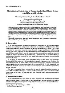
2. Finance-Based Scheduling When the cash is limited in a construction company, the project may be funded by bank overdrafts, especially line of credit agreement. Upon the line of credit agreement the contractor may borrow up to a specified amount of money on an as needed basis. The contractor pays interest on the amount of funds borrowed at any given time. In such case, the contractor must limit its debts within the available credit limit at any time during the execution stage. Finance-based scheduling modifies the start time of project activities and extends the total project duration (if needed), to limit the project’s negative cash flow within the available credit limit. The method helps to develop financially feasible schedules corresponding to desired credit limits. Control of the credit limit of a line of credit provides many benefits including negotiating lower interest rates with bankers, setting favorable terms of repayment, and reducing penalties incurred for any unused portions of overdraft cash (Elazouni and Gab-Allah, 2004). Developing schedules by finance-based scheduling method involves extending the initial schedule to meet the constraining cash flow and budget. In order to find (1) total duration, (2) required credit, and (3) financing cost of non-dominated schedules for a given project, devising initial and extended schedules are two primary steps. The initial schedule is basically a bar chart that portrays project activities against time disregarding any limitation in available resources. It must be analyzed to determine early start (ESk), early finish (EFk), and total float (TFk) of each activity. The total float represents the maximum shift in an activity without affecting project duration (Fig. 1(a)). Fulfilling the objectives of devising financially feasible schedules and minimizing project duration, according to different credit limits, necessitates developing an extended schedule. Devising a schedule that is constrained with a specified credit limit involves modification of initial schedule by extending the initial duration of the project (Fig. 1(b)). Extension increment and adjusted total float concepts were introduced by Elazouni and Gab-Allah (2004). Different extended schedules may be developed based on the initial schedule and trial extension increment (M). Any definite extension increment can transform the boundless solution space to a well-defined and more constrained one. The extension increment, as a definite value, is used to modify the total float of activities in the initial schedule. It extends the total float of activities resulting in adjusted total float (Jk) that allows the same extension in total duration of the project:
− 628 −
KSCE Journal of Civil Engineering
GA-Based Multi-Objective Optimization of Finance-Based Construction Project Scheduling
Fig. 2. Typical Cash Flow Profile of Period t for a Construction Project
Fig. 1. Initial and Extended Schedule of a Sample Project with Increment M
Jk = TFk + M
(1)
The adjusted total float defines the maximum possible shift in start time of an activity without affecting the total duration in the extended schedule. The M must be chosen with consideration to maximum allowable project extension time according to contractual and agreement’s terms. When the start time of an activity is shifted within its adjusted total float, then the same or greater shift must be assigned to the successor activities to preserve the logical precedence relationships among activities.
3. Cash Flow and Financial Terms When a construction company receives progress payment for a project, the released cash from the client has following three unique characteristics. First, the cash for the project is usually released only once during each period. Second, the owner may hold back part of the due payments in the form of retention, which will be released after the project completion. Third, a construction company can often defer paying some of the costs associated with the construction. Considering the above cash flow characteristics in progress payment projects, the manager must develop a cash inflowoutflow program. The cash inflow-outflow program consists of cost-loaded schedule, payment plan for the prepared cost-loaded schedule, and the payment received from the client. Vol. 14, No. 5 / September 2010
The financing cost of the project (i.e., interest charge of line of credit) must be included in the cash outflows. Fig. 2(a and b) present typical cash flow profiles in a period according to contractor perspective without and with considering financing cost, respectively. The effect of interest charge is determined based on the assumption that the contractor pays the interest charges due at the end of each period. Total project disbursement can be divided into two parts, direct cost and indirect cost. Direct cost of the project is sum of the costs related to material, labor, equipment, and subcontractors. Indirect cost encompasses fixed overhead and variable overhead. Fixed overhead costs are those tend to be fixed over a specific range of work volume. For example, if administrative office of the project currently has one salaried employee working as secretary, the cost of this employee is fixed over the volume of work that can be managed by him. But, variable overhead costs, such as utility costs in job site, personnel scheduling and management costs, taxes, and project insurance, vary with the volume of performed work. The equations in this section are presented according to the financial terminology used by Au and Hendrickson (1986) and the typical cash flow profile for construction projects applied in Elazouni and Gab-Allah (2004). Let the total direct cost in day i be represented by yi : yi =
ni
∑ ypi ; i = 1, 2, ..., T
(2)
p=1
in which ni is the number of activities whose duration overlaps with day i; ypi is the direct cost expenditure rate of activity p in day i; and T is the total duration of project. If Et stands for project total cost disbursement during a typical project period t:
− 629 −
Et =
m×t
∑
i = (m × (t – 1) ) + 1
( yi + OF ) + OVt
(3)
Habib Fathi and Abbas Afshar
where m is the number of days comprising a period; OF is the fixed overhead cost which is assumed to be fixed in each day i; and OVt is the variable overhead cost at period t which is considered to be a fixed percent of the total direct costs in relevant period. In order to calculate the payment amount Pt at the end of each period in periodic progress payment projects, the amount of retention (R) and profit and overhead markup (POM) must be defined. Retention is a percentage of each bill which clients often withhold to ensure the contractor completes the construction project. This portion of the progress payment will often be released when the job is completed. Profit and overhead markup is a percentage which companies commonly multiply to construction costs (direct costs) to get the bid price. Pt = ( 1 – R ) × ( 1 + POM ) ×
m×t
∑
yi
(4)
i = ( m × (t – 1)) + 1
The cumulative cash flow at the end of period t (for t ≥1) (disregarding interest charges) may be represented by Ft (Elazouni and Gab-Allah 2004): Ft = Nt – 1 + Et
(5)
Nt – 1 = Ft – 1 + Pt
(6)
in which Nt is the net cash flow at the end of period t after receiving a payment Pt disregarding interest charges; and Pt - 1 is the payment at the end of period t - 1. Let It represents the interest charges at the end of period t: –( Et + N'r – 1 ) It = –r ( Et + N't – 1 ) × ----------------------------Er – N't – 1 – γ
Fig. 3. Multi-objective Model Structure
(7)
where r is the interest rate per period; and γ is a very small positive real number to avoid the divided by zero case and also justify the situation that Et =0 and N't- 1 >0. The term [ –( Et + N'r – 1 ) / ( Er – N't – 1 – γ )] can only be equal to {-1, 0} and adjusts the equation to take care of the positive values for (Et + N't-1). In this case, the contractor borrows no money from the financial institution and hence pays no interest at the end of period. It must be mentioned that [ ] denotes the floor function which maps a real number to the next smallest integer. Note that the above calculation is based on the assumption that contractor pays the interest charges at the end of each period. The actual cumulative cash flow at the end of period t which comprises interest charges, F 't , may be defined as the sum of Ft and the interest charge for that period, It, as: F't = Ft + It
(8)
As illustrated in Fig. 2(b), N 't , the net cash flow until the end of period t including accumulated interest charges can be calculated by: N 't = F 't + Pt
(9)
The calculation of required credit and financing cost of any conceivable schedule according to extended schedule, are
founded on the above equations. Based on the defined concept and mathematical representation of the cash balances, the structure of the proposed multi-objective model is summarized as Fig. 3.
4. Pareto Front Searching Process; GA Approach Multi-Objective optimization deals with more than one objective function which may be in conflict with each other. In fact there may not necessarily exist a fully superior solution corresponding to all objectives. Therefore, the best solution of problem has to be selected by decision maker according to a specific order of importance of the objectives from a set of optimal nondominated solutions referred to as Pareto front. Moreover, in a multi-objective optimization it is essential to maintain a diverse set of solutions in the non-dominated front. The Pareto front consists of all non-dominated solutions for the given multiobjective problem. The concept of domination between two solutions can be represented as: A solution x1 is said to dominate the solution x2, if not only the solution x1 be no worse than x2 in all objectives but also the solution x1 be strictly better than x2 in at least one objective. The main objective of the proposed model is to find the non-dominated solutions with minimum total duration of the
− 630 −
KSCE Journal of Civil Engineering
GA-Based Multi-Objective Optimization of Finance-Based Construction Project Scheduling
project, required credit from bank, and total financing cost. In order to apply NSGA-II rules for non-dominated solutions finding process, first of all, the initial and the extended schedules have to be developed according to Fig. 1 with the aim of determination the possible solution space. Then, six primary steps of NSGA-II algorithm are performed including: setting the chromosome structure; generating an initial population of chromosomes; performing offspring generation operators; evaluating each chromosome based on defined objectives; performing a non-dominated sorting and identifying different fronts; crowding distance sorting and setting the new population. The chromosome structure is set as a string of elements which is depicted in Fig. 4. It shows a sample chromosome related to the project in Fig. 1. Each gene can take a number between 0 to adjusted total float of the relevant activity. In the next two steps (i.e., generating initial population and performing genetic operators), three major problems were detected in applying the basic procedures of GA which have been defined in the literature. First, precedence relationship may be violated very often. Crossover and mutation operators in the basic GA system alter the contents of genes, thus causing violation of the precedence constraint. In other words, most new chromosomes generated from crossover and mutation may become infeasible solutions. Second, the diversity of optimal-Pareto front which is a basic goal for multiobjective optimization was not fulfilled very well. The acquired non-dominated solutions mostly concentrated on the region with greater total duration, missing the solutions with lower duration. Third, the basic GA contained two redundant operations; it allowed two identical parents to swap genetic material in crossover. Also, acquired offspring from two dissimilar parents, may be similar to their parents. These operations should be eliminated. In order to enhance the performance of the model and surmount the aforementioned problems, three modifications are proposed and implemented in this paper. The improved initial population generating procedure, modified crossover, and revised mutation highly enhanced the performance of the algorithm. The resulted Pareto front approached to the actual non-dominated
Fig. 4. Chromosome Structure Vol. 14, No. 5 / September 2010
solutions with well diversity. The following sections describe these modifications. The paper uses the project depicted in Fig. 1 to exemplify the modified procedures. 4.1 Improved Initial Population Generating Procedure The adjusted total float of activities in extended schedule is used to generate the initial population of chromosomes. The improved procedure for generation of initial population has the following steps: 1. select randomly an activity (i.e., a gene); 2. select a random shift value between 0 to adjusted total float of the selected activity in step 1; 3. select randomly the direction of movement (left or right) from the selected gene in step 1; 4. if the left (right) direction is selected in step 3, check whether the shift value is assigned to the left (right) gene’s successors (predecessors) or not. if none of them has been shifted→select 0≤Shift≤Jg if shift value is assigned at least for one of them⇒then select ⎧ for left 0 ≤ Shift ≤ MISS – Fg ⎨ ⎩ for right MAS F – Sg ≤ Shift ≤ Jg in which Shift is a random number between specified limits; Jg is the adjusted total float for the current gene; MISS is the minimum modified start time of successors; MASF is the maximum modified finish time of predecessors; Sg is the start time of the current gene based on the initial schedule; and Fg is the finish time of the current gene based on the initial schedule. Repeat this procedure for all the genes which are in the left (right) side of the selected gene in step 1 respectively; 5. repeat step 4 for the opposite direction which is selected in step 3. Table 1 illustrates the proposed procedure for gene number 4, left direction, with selected shift value of 3 units. The generated chromosome is portrayed in Fig. 5. 4.2 Improved Crossover Crossover is a stochastic operator that allows information exchanges between chromosomes. It allows selected individual solutions to trade characteristics by exchanging parts of strings. Fig. 6 illustrates that two strings (parent 1 and 2) are randomly selected and broken at a random point (at gene 3), and after the exchange two new strings (offspring 1 and 2) are generated. Splitting the parent chromosomes from one point entitled as single-point crossover. After the single-point crossover, an additional operation is introduced to ensure that the offspring are still feasible solutions. This operation is explained as: 1. select randomly an activity (i.e., a gene); maintain its content, and mark this gene as a repaired gene; 2. select randomly the direction of movement (left or right) from the selected gene in step 1; 3. if the left (right) direction is selected in step 2, check whether the left (right) gene has successor (predecessor) or not. If it
− 631 −
Habib Fathi and Abbas Afshar
Table 1. An Example for Improved Initial Population Generating Procedure Left Activities (Gene) Number
Successor Activities
MISS
Lower and Upper Limit for Shift Value
Selected Shift value
3
7
-
0, 6
2
2
3, 4
6
0, 4
1
1
3, 4
6
0, 2
0
Right Activities (Gene) Number
Predecessor Activities
MASF
Lower and Upper Limit for Shift Value
Selected Shift value
5
4
9
3, 4
3
6
4
9
3, 6
5
7
3, 5
12
3, 4
3
0 ≤ Cg ≤ MISmS – Fg → maintain its content and mark it else 0 ≤ Shift ≤ MISmS – Fg → then mark it MASmF – Sg ≤ Cg ≤ Jg for right if → maintain its content and mark it else MASmF – Sg ≤ Shift ≤ J g → then mark it where MISmS is the minimum modified start time of successors which were marked as a repaired gene; MASmF is the maximum modified finish time of predecessors which were marked as a repaired gene; and Cg is the content of the current gene. Repeat this operation for all the genes which are in the left (right) side of the selected gene in step 1 respectively; 4. repeat step 3 for the opposite direction which is selected in step 2. A sample crossover which creates illegal offspring is displayed in Fig. 6, and the steps of the repairing process are illustrated in Table 2. The selected gene for repairing is 4, and the selected direction is right. Fig. 7 demonstrates the repaired chromosome after the operation. for
Fig. 5. Sample Generated Chromosome based on Example
left
if
Fig. 6. Basic Crossover Operation
does not have any, maintain the content of it and mark it as a repaired gene; if it has successor (predecessor):
4.3 Improved Mutation Mutation, by occasional random alteration of the value with respect to gene’s position, is used for searching in unexplored
Table 2. Repairing Process for the Acquired Illegal Chromosome in Sample Crossover Right Activities (Gene) Predecessor Activities Number 5
4
Marked Predecessors
MASF
Lower and Upper Limit for Shift Value
Selected Shift value
4
7
1, 4
Maintained
6
4
4
7
1, 6
Maintained
7
3, 5
5
10
1, 4
Maintained
Left Activities (Gene) Number
Successor Activities
Marked Successors
MISS
Lower and Upper Limit for Shift Value
Selected Shift value
3
7
7
11
0, 4
3
2
3, 4
3,4
5
0, 3
Maintained
1
3, 4
3,4
5
0, 1
0
− 632 −
KSCE Journal of Civil Engineering
GA-Based Multi-Objective Optimization of Finance-Based Construction Project Scheduling
Therefore, the objectives of the model which must be minimized may be represented mathematically as: ⎧ f1 = max ( mFk ) k = 1, 2, ..., n ⎪ minimize ⎨ f2 = min ( F't ) t = 1, 2, ..., tf ⎪ ⎩ f3 = FC s.t. → Network Logic
Fig. 7. Repaired Offspring
portions of solution space and keeping the diversity in population. To perform mutation, one string from the population is randomly selected and one of its genes is picked by chance. Then, the information in the selected gene is changed arbitrarily. The random changes introduced by the basic mutation operator may invalidate the precedence relationship. To maintain the precedence and produce legal chromosomes, the same operation as the repairing process in improved crossover section is employed. Besides, another modification is performed in chromosome selection process for mutation. The proposed algorithm prohibits the selection of chromosomes in the first non-dominated front at previous generation for producing the offspring of next generation. Besides, when the members of acquired first non-dominated front at previous generation exceeds the population size, which means the whole parent members of next generation are from this front, only chromosomes from second mid of next generation’s parents population are selected for mutation. Note that this modification ensures that model does not lose the acquired best solutions till now, because of alteration of them by mutation process. Using the improved initial population generating procedure, a random parent population P0 of size N is created. Then, single point improved crossover and mutation operators are applied on P0 to create a offspring population Q0 of size N. In general, the tth generation of the proposed algorithm can be described as: Following the formation of parent population (Pt) and offspring chromosomes (Qt), a combined population ( Rt = Pt ∪ Qt ) must be formed. Since the size of each one is same (N), the combined population size will be 2N. Then, the fitness of every individual in Rt is evaluated. Intending to simultaneously optimize three objectives (i.e., total project duration, required credit, and total financing cost), fitness evaluation necessitates calculation of the amount of each objective for each member. The total duration is determined as the greatest modified finish time for all activities (i.e., early finish based on the initial schedule plus the shift assigned to that activity, mFk). The maximum negative cash flow represents the required credit that must be financed by bank overdrafts. Finally, as defined earlier the total financing cost FC can be calculated as: t E –( Et + N't – 1 ) ⎞ FC = r -----1 + ∑ –r ⎛ ( Et + N't – 1 ) × ---------------------------⎝ Et – N't – 1 – γ ⎠ 2 t=2
(10)
tf = tp + tr
(11)
f
in which tp is the total number of periods in project duration; and tr is the number of periods from bill submission to payment release from the client. Note that advance payment and mobilization cost are assumed to be zero in Eq. (10). Vol. 14, No. 5 / September 2010
(12)
As F 't is negative in given periods, min(F 't) represents the maximum negative cash flow and is equal to the amount of credit that the contractor needs to procure. Taking the absolute value eliminates the negative sign for the minimization process. Then, the population Rt is sorted according to non-domination concept. In order to identify solutions of the first non-dominated front (λ1), the first member is directly entered in λ1. The next members are compared with the solutions of λ1 respectively. If the solution dominates any member of λ 1, the dominated solution will be replaced by the dominant. Otherwise, if the solution neither dominates nor be dominated by the members of λ1, it will be added to λ1. This process is continued to find all members of the first non-dominated level. In order to find the individuals in the next non-dominated front, the solutions of the first front are omitted temporarily and the above procedure is repeated. Solutions belonging to the best non-dominated set are of best solutions in the combined population and must be emphasized more than any other solution in Rt (Deb et al., 2002). To perform the emphasis, the paper uses crowded-comparison operator to select the members of new population. This operator requires both the rank and crowded distance (a measure of density of solutions in the neighborhood) of each solution in the population. The solutions with lower rank have priority for selection. Among solutions from same rank, greater crowding distance determines the superior solution to be selected. The new population is then used in the next iteration of the algorithm. Commonly, the algorithm terminates when either a maximum number of generations has been produced, or a satisfactory fitness level has been reached for the population.
5. Model Verification To verify the structure and performance of the proposed multiobjective finance-based scheduling model, a test network with 8 activities was designed by the authors as depicted in Fig. 8. This test network was solved by means of complete enumeration in solution space for two objectives (i.e., total duration and required credit). The two objective problem was selected to reduce the number of non-dominated solutions so that their comparison can be made in depth. Its true Pareto front which includes all non-dominated solutions was obtained by checking all possible solutions. The extension increment was assumed as 10 working days. Other parameters were set as: OF =10 dollars per day, OV =10%, R=10%, POM=20%, r=0.3% per period, and m=5 days. To find the true Pareto front, adjusted total float was calculated for each activity. Subsequently, any conceivable shifting com-
− 633 −
Habib Fathi and Abbas Afshar
Fig. 8. The Benchmark Network
from the proposed model. As Table 3 illustrates, the solutions from the model fulfill the two basic goals of multi-objective optimization process (i.e., convergence to the Pareto-optimal set and maintenance of diversity in solutions). The convergence is evaluated by a performance metric (γ ), which measures the extent of convergence to a known set of Pareto-optimal solutions. The γ for each solution is the Euclidean distance between the solution and the corresponding solution in Pareto-optimal set. The average normalized (the calculated distance for each objective is divided by the related amount in optimal-Pareto set for normalization) γ for the network is 0.0041 and the variance is 0.0000829. In fact, 7 solutions out of 11 solutions resulted in exactly the same non-dominated ones. Remaining 4 nondominated solutions differ from the true ones by less than 2.5 percent. The second goal can be assessed by the extent of spread achieved among the solutions obtained. With respect to
bination was enumerated by alteration of the shift value within 0 to Jk for each activity. It determines the entire search space of the benchmark problem. Among the combinations, there are some members which violate the precedence relationship and cannot be handled. Disregarding them, calculation of total duration and required credit for legal solutions comprise the next step. Afterward, sorting procedure was done according to the nondomination concept and the first rank of non-dominated solutions forms the true Pareto front. Then, the benchmark problem was tailored and solved with the proposed model in which the modeling dimension was reduced from 3 to 2 of disregarding the financing cost. Through a comprehensive sensitivity test the tunable parameters of the GA based model were finalized as 100, 3%, and 300 for population size, mutation percent, and number of generations, respectively. Table 3 compares the true Pareto front with solutions acquired
Table 3. Comparison of the True Pareto Front with Solutions Acquired from the Proposed Model for Benchmark Problem (A week-later payment) Non-dominated Solutions From True Pareto Front Total Required Duration Credit
Acquired Solutions By The Proposed Model
Activity Shift Value 1
2
3
4
5
6
7
8
Total Required Duration Credit
Activity Shift Value 1
2
3
4
5
6
7
8
Credit Difference (%)
22
66314.97
0
0
1
5
0
1
0
0
22
66314.97
0
0
1
5
0
1
0
0
0
23
64988.52
0
0
2
5
1
2
1
1
23
64988.52
0
0
2
5
1
2
1
1
0
24
58362.09
0
0
3
5
2
3
2
2
24
58362.09
0
0
3
5
2
3
2
2
0
25
54196.82
0
0
2
5
3
3
3
3
25
54196.82
0
0
2
5
3
3
3
3
0
26
53261.38
2
1
4
9
2
5
4
4
26
53261.38
2
1
4
9
2
5
4
4
0
27
53048.9
2
2
4
10
2
6
4
5
27
53062.12
2
1
4
9
2
5
4
5
0.0249
28
52100.97
1
4
1
10
6
7
6
6
28
52101.35
2
2
3
10
6
7
6
6
0.0007
29
48727.77
0
4
8
4
7
8
7
7
29
49743.95
2
2
4
10
5
8
7
7
2.085
30
45351.04
0
4
4
10
7
9
8
8
30
45351.04
0
4
4
10
7
9
8
8
0
31
42570.16
7
0
7
14
5
10
9
9
31
43594.91
9
0
9
14
2
10
9
9
2.407
32
42476.51
9
0
9
15
4
11
9
10
32
42476.51
9
0
9
15
4
11
9
10
0
− 634 −
KSCE Journal of Civil Engineering
GA-Based Multi-Objective Optimization of Finance-Based Construction Project Scheduling
extension increment of 10 days, both true Pareto front and results of the model comprise 11 non-dominated points. So, the diversity of solutions is totally fulfilled. It worth to mention that entire search space includes approximately 405 million solutions from which only 34 millions are legal solutions. The proposed algorithm with 30000 function evaluations resulted in 11 non-dominated solutions from which 7 were exactly the same as the global ones. It means that the model at most by evaluation of 0.007 percent of the solution space produced quite desirable results.
6. Application of the Model A construction project case example (derived from Hegazy 1999) is used to further demonstrate the performance of the proposed multi-objective model on larger networks. The example is defined with three objectives of total duration, required credit, and financing cost. Fig. 9 displays the original network of the project consisting of twenty activities. The duration, total float, and direct cost per day of activities are displayed at the same figure. The payment is made one period after submission of the periodic pay request, with no advance payment. Besides, M=10 days, OF =10 dollars per day, OV =10%, R=10%, POM=20%, r=1% per period, and m=5 days are considered as the model parameters. According to the network analysis and selected extension increment, the solution apace comprises more than 1022 members. The formulated model was solved using MATLAB and the results are listed in Table 4. To make the presentation of the relationships between variables more clear, Fig. 10(a, b, and c) compare the trends of Pareto front for two variables at a time. It is important to note that GA parameters were set as 200, 300, 3 for population size, number of generations, and mutation percent, respectively. Offering different possible non-dominated solutions, proposed model facilitates the process of selecting the most appropriate cash provision option for construction company.
The project manager can observe the overall influence on project performance while changing acceptable extended project duration, and thus adopt the most beneficial actions (Fig. 10(a)). For example, if the contractor does not have authorization to enlarge the original project duration (i.e., 32 days), credit amount of at least $66476.78 should be provided. Whereas, applying 3 days extension will decrease the amount to $58717.38. And, in case of permission for 10 days extension, the minimum allowable credit for the project execution will be $48142.96 which shows 28 percent reduction compared to the first manner. Therefore, the lower the available credit, the larger the project execution time. On the other hand, in the solutions possessing a specific duration, setting tighter amounts for available credit increases financing cost and results in lower profit for the company (Fig. 10(b)). According to the results shown in Table 4, accumulated interest charges and required credit for solution number 48 is $3044.487 and $79831.93 respectively; while in solution number 35, required credit reduction to $61287.84 brings about financing cost growth to $3064.228. The main reason may lie in the retention amount. Comparing the shift values which are assigned to the project activities according to these solutions reveals that the volume of work scheduled for execution at early periods of solution number 35 is more than the other solution. As the client withholds a percentage of each bill in the retention form and the contractor must pay interest on this portion till the end of the project, it signifies to higher amount of payable interest charges for the solution number 35. If the contractor desires to earn higher profits considering a particular project execution time, the firm ability to provide cash should be strengthened. However, financial institutions usually limit the available credit based on different measures. The project manager must always negotiate with bankers to gain further credits and lower the interest rate. Considering the resulted Pareto front (Fig. 10(c)), the solutions can be divided to three groups. The first one includes the solutions possessing total duration from 32 to 35. Compared to other solutions, they have lower duration, larger required credit,
Fig. 9. Construction Project Case Example Network Vol. 14, No. 5 / September 2010
− 635 −
Habib Fathi and Abbas Afshar
Table 4. Non-dominated Solutions for Case Example Project Number 1 2 3 4 5 6 7 8 9 10 11 12 13 14 15 16 17 18 19 20 21 22 23 24 25 26 27 28 29 30 31 32 33 34 35 36 37 38 39 40 41 42 43 44 45 46 47 48 49 50 51 52 53 54 55 56 57 58 59 60 61 62 63 64
Duration 32 32 32 32 32 32 32 32 32 32 32 32 32 32 32 32 32 32 32 33 33 33 33 33 33 33 33 33 33 33 33 33 33 33 34 34 34 34 34 34 34 34 34 34 34 34 34 34 35 35 35 35 35 35 35 35 35 35 35 35 35 35 35 35
Required Credit 66476.78 67096.01 68095.79 68374.99 69662.26 70966.11 71333.06 73092.21 73955.92 74387.78 75251.48 76547.04 77410.75 77788.44 78240.36 79931.12 81694.45 82055.02 84214.28 63311.27 63842.63 64345.49 64416.28 64572.69 65284.04 65969.3 66059.76 66923.47 67616.45 69775.71 71255.74 74923.99 77460.39 80977.75 61287.84 61662.01 62722.85 63680.83 63994.64 64565.97 67287.79 67787.94 71172.02 73027.6 75447.99 77661.25 78492.45 79831.93 58717.38 58872.03 59379.22 59873.95 61133.24 61492.35 62085.23 62969.38 63541.71 63695.18 63985.94 65948.11 68035.29 68879.24 72704.78 73035.06
Financing Cost 3065.346 3064.577 3064.314 3063.546 3062.799 3062.624 3061.482 3060.714 3060.407 3060.253 3059.946 3059.485 3059.177 3057.16 3056.589 3055.821 3054.603 3053.835 3053.067 3070.833 3070.248 3069.737 3068.038 3065.601 3059.198 3059.026 3058.737 3058.429 3056.22 3055.452 3054.909 3051.003 3049.341 3048.679 3064.228 3063.787 3062.756 3062.322 3061.477 3056.404 3055.288 3054.191 3050.528 3047.705 3047.526 3046.739 3045.293 3044.487 3048.566 3045.927 3044.419 3042.516 3041.16 3040.868 3039.715 3038.947 3038.149 3037.822 3036.338 3033.662 3032.894 3030.733 3030.677 3028.462 − 636 −
Number 65 66 67 68 69 70 71 72 73 74 75 76 77 78 79 80 81 82 83 84 85 86 87 88 89 90 91 92 93 94 95 96 97 98 99 100 101 102 103 104 105 106 107 108 109 110 111 112 113 114 115 116 117 118 119 120 121 122 123 124 125 126 127 128
Duration 36 36 36 36 36 37 37 38 38 38 38 38 38 38 38 38 38 39 39 39 39 39 39 39 39 39 39 39 39 39 39 40 40 40 40 40 40 40 40 40 40 40 40 40 40 40 40 40 40 40 41 41 41 41 41 42 42 42 42 42 42 42 42 42
Required Credit 57873.84 58454.42 58935.02 60307.47 61005.63 56408.23 56625.19 54222.41 54250.23 54462.83 54750.31 54813.86 55186.31 56055.58 56434.41 57983.65 58344.12 51489.94 51950.26 52379.93 52585.01 52662.96 53634.02 53678.67 54758.21 55622.02 56146.41 56359.5 57597.13 59900.26 60692.99 50913.92 51215.19 51534.33 52108.63 53256.7 57337.99 58440.31 58934.34 59763.08 60982.45 62112.01 62952.36 62958.79 63111.96 64541.44 65126.45 68990.76 72209.47 81824.08 49995.13 50282.7 50619.75 50813.07 51354.54 48142.96 48179.22 48345.25 48345.83 48592.48 49032.43 49430.93 49812.1 50966.66
Financing Cost 3122.67 3116.547 3115.475 3114.233 3113.417 3110.826 3103.651 3105.115 3104.431 3100.983 3098.761 3093.825 3092.856 3087.48 3083.162 3081.097 3080.391 3094.094 3093.735 3093.706 3091.65 3091.463 3090.29 3082.258 3081.782 3081.587 3079.815 3076.81 3076.474 3074.048 3073.864 3090.582 3088.019 3076.944 3076.478 3069.023 3067.453 3066.782 3062.919 3062.389 3061.86 3058.732 3056.618 3056.07 3055.299 3051.246 3050.636 3049.171 3046.635 3027.263 3150.733 3141.531 3138.885 3138.101 3132.881 3144.641 3143.572 3142.585 3140.973 3128.11 3127.438 3125.848 3123.489 3117.467
KSCE Journal of Civil Engineering
GA-Based Multi-Objective Optimization of Finance-Based Construction Project Scheduling
A number of what-if scenarios can be tested for the analyzed construction project, as shown in Table 5. The scenarios evaluated for different sets of importance coefficient for the objectives, which were selected to find optimal solutions. In these sets, the order of objectives signifies their importance for the decision maker. In the second one, for example, the project manager has obligation to select the option with the minimum duration (32 days). There are 19 solutions which satisfy the first desire. So, the next objective (i.e., financing cost) must be checked. Accordingly, the solution number 19 with lowest financing cost ($3053.067) is the optimum solution based on the project manager’s desires.
7. Conclusions
Fig. 10.The Relationship between Each Two Variables in Acquired Pareto Front
and lesser financing cost. According to these options, the execution of the project will be completed in 7th period. In the second group, total duration of the solutions range from 36 to 40 which signifies the completion of the project at 8th period. Although financing cost of the options from one group changes slightly, Fig. 10(c) clearly shows a considerable difference in financing cost of the solutions from the first and second groups. The main reason may lie in the fact that members of the second group need 8 periods while the first ones require 7. The same scenario acts on the solutions with 41 and 42 days duration which comprise the third group. They have the least required credit and the highest financing cost.
This paper presented a robust and efficient multi-objective optimization model of finance-based scheduling using the general concept of non-dominated sorting genetic algorithm with elitism. The model may be applied in devising a realistic plan for cash providing alternatives and negotiation for establishing good bank overdrafts. It generates a Pareto front, comprises nondominated schedules, based on total duration of project, required credit that must be procured by bank overdrafts, and financing cost as objectives of the model. To improve the accuracy, diversity, and efficiency of the basic non-dominated sorting GA, a number of modifications were introduced. The results of the model displayed that the proposed modifications were quite efficient in locating a Pareto front comparable with the true front in limited number of function evaluation in a bi-objective test problem. The project manger can use some what-if scenarios in order to find the optimum cash providing option based on specific importance which assigns to each objective. The model may be improved by considering some real involved project’s restrictions. For instance, the model can be expanded to consider (1) different available and/or presumed implementation option for each activity; (2) client’s budget limitation, and cash release conditions; or (3) uncertainties associated with interest rate and other financial terms. Also, more research and development efforts are needed to ensure a steady performance of the model when applying to large-scale projects. Another important feature of financing in construction projects is that contractors usually deal with the issue at the corporate level rather than at project level. Accordingly, they may establish credit lines to procure cash for all ongoing projects.
Table 5. Sample What-if Scenarios Scenario
Importance of Objectives
Total Duration
Required Credit
Financing Cost
1
time > credit > financing cost
32
66476.78
3065.346
2
time > financing cost > credit
32
84214.28
3053.067
3
credit > time > financing cost
42
48142.96
3144.641
4
financing cost > time > credit
40
81824.08
3027.263
Vol. 14, No. 5 / September 2010
− 637 −
Habib Fathi and Abbas Afshar
Notation Cg = Content of the current gene in repair procedure for crossover and mutation Et = Construction disbursement in period t Fg = Finish time of the current gene based on initial schedule F't = Cumulative cash flow at end of period t, including accumulated interest charges Ft = Cumulative cash flow at end of period t just before receiving payment Pt disregard to interest charges FC = Total financing cost of a solution It = Interest charges at end of period t Ja = Adjusted total float for the current gene Jk = Adjusted total float of each activity based on extended schedule M = Extension increment in extended schedule MASF = Maximum modified finish time of predecessors of the current gene MASmF = Maximum modified finish time of predecessors of the current gene which were marked as a repaired gene MISS = Minimum modified start time of successors of the current gene MISmS = Minimum modified start time of successors of the current gene which were marked as a repaired gene m = Number of days comprising period mFk = Modified finish time of activity k Nt = Cumulative net cash flow until period t disregard to interest charges N't = Cumulative net cash flow until period t including accumulated interest charges ni = Number of activities having durations overlapping with day i OF = Fixed overhead cost at each day OVt = Variable overhead cost at period t POM = Profit and overhead markup percent Pt = Receipt from owner payment at end of period t R = Retention percent r = Interest rate per period Sg = Start time of the current gene based on initial schedule T = Total project duration TFk = Total float of each activity tp = Total number of periods in project duration tr = Number of periods from bill submission to payment release from the client
References Abudayyeh, O. Y. and Rasdorf, W. J. (1993). “Prototype integrated cost and schedule control system.” J. Comp. in. Civ. Engrg., ASCE, Vol. 7, No. 2, pp. 181-199. Ashley, D. B. and Teicholz, P. M. (1977). “Pre-estimate cash flow analysis.” J. Constr. Div., ASCE, Vol. 102, No. 3, pp. 369-379. Au, T. and Hendrickson, C. (1986). “Profit measures for construction projects.” J. Constr. Eng. Manage., Vol. 112, No. 2, pp. 273-286.
Chen, H. L. and Chen, W. T. (2000). “An interactive cost-schedule/ payment schedule integration model for cash flow forecasting and controlling.” Proc. 17th int. Symp. on Automation and Robotics in Construction, Taipei, Taiwan, pp. 659-663. Deb, K. (2002). Multi-objective optimization using evolutionary algorithms, Wiley, New York. Deb, K., Pratap, A., Agarwal, S., and Meyarivan, T. (2002). “A fast and elitist multiobjective genetic algorithm: NSGA-II.” IEEE Transactions on Evelutionary Computation, Vol. 6, No. 2, pp. 182-197. Elazouni, A. and Abido, M. (2009). “Finance-based scheduling of multiple construction projects using multiobjective evolutionary algorithms.” 2nd International Construction Specialty Conference, Canadian Society of Civil Engineers. Elazouni, A. and Gab-Allah, A. (2004). “Finance-based scheduling of construction projects using integer programming.” J. Constr. Eng. Manage., Vol. 130, No. 1, pp. 15-24. Elazouni, A. and Metwally, F. G. (2005). “Finance-based scheduling: Toll to maximize project profit using improved genetic algorithm.” J. Constr. Eng. Manage., Vol. 131, No. 4, pp. 400-412. Elazouni, A. and Metwally, F. G. (2007). “Expanding finance-based scheduling to devise overall-optimized project schedules.” J. Constr. Eng. Manage., Vol. 133, No. 1, pp. 86-90. Fathi, H. and Afshar, A. (2008). “Financed-based scheduling for construction projects with improved ILP model.” CSCE 2008 Annual Conference, Quebec City. Hegazy, T. (1999). “Optimization of resource allocation and leveling using genetic algorithms.” J. Constr. Eng. Manage., Vol. 125, No. 3, pp. 167-175. Jang, H. S. (2004). “Genetic algorithm for construction space management.” KSCE J. Civil Eng., Vol. 8, No. 4, pp. 365-369. Kenley, R. and Wilson, O. D. (1989). “A construction project net cash flow model.” Constr. Manage. Econom., Vol. 7, No. 1, pp. 3-18. Kirkpatrick, H. H. (1994). “Using computer modeling for cash flow projection.” Real State Finance Journal., Vol. 10, No. 2, pp. 93-96. Li, H. and Love, P. (1997). “Using improved genetic algorithms to facilitate time-cost optimization.” J. Constr. Eng. Manage., Vol. 123, No. 3, pp. 233-237. Liu, S. S. and Wang, C. J. (2008). “Resource-constrained construction project scheduling model for profit maximization considering cash flow.” Automation in Construction, Vol. 17, No. 8, pp. 966-974. Navon, R. (1994). “Cost-schedule integration for cash-flow forecasting.” Proc. 1st Congress on Computing in Civil Engineering., ASCE, New York, pp. 1536-1539. Navon, R. (1995). “Resource-based model for automatic cash-flow forecasting.” Constr. Manage. Econom., Vol. 13, No. 6, pp. 501-510. Navon, R. (1996). “Company-level cash flow management.” J. Constr. Eng. Manage., Vol. 122, No. 1, pp. 22-29. Park, H. K. (2004). “Cash flow forecasting in construction project.” KSCE J. Civil Eng., Vol. 8, No. 3, pp. 265-271. Peterson, J. (2005). Construction accounting and financial management, Pearson Education, New Jersey. Que, B. C. (2002). “Incorporating practicability into genetic algorithmbased time-cost optimization.” J. Constr. Eng. Manage., Vol. 128, No. 2, pp. 139-143. Slovin, M. B. and Young, J. E. (1990). “Bank lending and initial public offerings.” Journal of Banking and Finance., Vol. 14, No. 4, pp. 729-740. Zheng, D., Thomas, S., and Kumaraswamy, M. (2004). “Applying a genetic algorithm-based multiobjective approach for time-cost optimization.” J. Constr. Eng. Manage., Vol. 130, No. 2, pp. 168-176.
− 638 −
KSCE Journal of Civil Engineering