Gabor Filters as Feature Images for Covariance Matrix on ... - CiteSeerX

Gabor Filters as Feature Images for Covariance Matrix on Texture Classification Problem Jing Yi Tou1, Yong Haur Tay1, and Phooi Yee Lau1,2 Computer Vision and Inteligent Systems (CVIS) group, Universiti Tunku Abdul Rahman (UTAR). 9, Jalan Bersatu 13/4, 46200 Petaling Jaya, Selangor, Malaysia [email protected] 2 Instituto de Telecomunicações. Av. Rovisco Pais, 1049-001 Lisboa, Portugal [email protected] 1

Abstract. The two groups of popularly used texture analysis techniques for classification problems are the statistical and signal processing methods. In this paper, we propose to use a signal processing method, the Gabor filters to produce the feature images, and a statistical method, the covariance matrix to produce a set of features which show the statistical information of frequency domain. The experiments are conducted on 32 textures from the Brodatz texture dataset. The result that is obtained for the use of 24 Gabor filters to generate a 24 × 24 covariance matrix is 91.86%. The experiment results show that the use of Gabor filters as the feature image is better than the use of edge information and co-occurrence matrices.

1 Introduction Texture classification has been studied for years because of its usefulness in many computer vision applications. In these applications, the texture analysis helps to recognize the images through its texture information [1], such as wood species recognition [2][3], rock classification [4], face detection [5] and etc. The texture classification methods can be divided into five main groups in general, namely the; 1) structural; 2) statistical; 3) signal processing; 4) model-based stochastic [1] and; 5) morphology-based methods [6]. The statistical and signal processing methods are most widely used because they can be used on general textures while other methods have more restriction on the characteristics of the textures that they can be implemented on. Some of these methods can be combined for better performance. In our previous work [7], a combination of a statistical method, the grey level cooccurrence matrices (GLCM) and a signal processing method, the Gabor filters is used. The combination here is to append both the GLCM and Gabor features as a single feature vector. In this paper, we propose a combination method where the signal processing method, the Gabor filters are used as the feature images to generate the covariance matrix which is a statistical method. Section 2 shows the Gabor filters and the covariance matrix algorithms used in the paper. Section 3 shows the dataset and settings used in the experiments conducted.

Section 4 shows the experiment results and analysis. Section 5 shows the conclusion and future works.

2 Gabor Filters and Covariance Matrix The Gabor filters is a type of signal processing method while the covariance matrix is a statistical method. In this paper, the Gabor filters are used as feature images, which are images or two-dimensional matrices produced by a feature extraction algorithm, that are used to generate a covariance matrix. 2.1 Gabor Filters The Gabor filters is also known as the Gabor wavelets [5]. The method extracts features through the analysis of the frequency domain rather than the spatial domain. The Gabor filters is represented by Equation (1) where x and y represent the pixel position in the spatial domain, 0 represents the radial center frequency, represents the orientation of the Gabor direction, and  represents the standard deviation of the Gaussian function along the x- and y- axes where x = y = .

  x, y ,  0 ,   





1 2 2 exp  x cos   y sin     x sin   y cos   / 2 2 2 2  exp i0 x cos   0 y sin    exp  02 2 / 2









(1)

The Gabor filter can be decomposed into two different equations, one to represent the real part and another to represent the imaginary part as shown in Equation (2) and Equation (3) respectively [5] while it is illustrated in Figure 1.

r x, y, 0 ,  



  x 2  y  2  2 2   cos 0 x  e 0 / 2 exp   2 2     1

2

 i  x, y ,  0 ,   

  x  2  y  2    sin 0 x exp   2 2 2     1

where x' = x cos + y sin

y' = -x sin + y cos



(2)

(3)

Fig. 1. Real part (left) and imaginary part (right) of a Gabor filter [8]

In this paper, we used  =  / 0. Gabor features are derived from the convolution of the Gabor filter and image I as shown in Equation (4) [5].

CI  I x, y  x, y,0 , 

(4)

The term (x, y, 0, ) of Equation (4) can be replaced by Equation (2) and Equation (3) to derive the real and imaginary parts of Equation (4) and is represented by CIr and CIi respectively. The real and imaginary parts are used to compute the local properties of the image using Equation (5) [5].

CI ( x, y, 0 , ) 

Cr I

2

 Ci I

2

(5)

The convolution is performed using a fast method that differs from the traditional convolution achieved through scanning windows by applying a one time convolution with Fast Fourier Transform (FFT), point-to-point multiplication and Inverse Fast Fourier Transform (IFFT). It is performed on different radial center frequencies or scales, 0 and orientations, . In this paper, the radial center frequencies and orientations are represented by m in Equation (6) where n  {0, 1, 2} and m  {0, 1, 2, …, 7} [5].

n 

 2 2

n

m 

 8

m

(6)

2.2 Covariance Matrix A covariance matrix shows the covariance between values. In this paper, we use the fast covariance matrix calculation using integral images that is proposed in [9] to

generate the covariance between different feature images to be used as the features for our algorithm. The covariance matrix can be represented as.

CR 

1 n z k   z k   T  n  1 k 1

(7)

where z represents the feature point and  represents the mean of the feature points for n feature points [9]. Integral images are used for faster computation. They will pre-calculate the summations for each pixel of the images from the origin point, so it is faster for the calculations of the sum for a region within the images. The calculations of the term P and Q which are two tensors for the fast calculation of the covariance matrix are shown below:

Px, y, i  

 F x, y, i 

i  1...d

x x, y  y

Qx, y , i, j  

 F x, y, i F x, y, i 

i, j  1...d

x  x , y  y 

(8)

(9)

where F represents the feature images and d represents the dimension of covariance matrix which is also the number of feature images. The covariance matrix is then generated using P and Q where x, y  is the upper left coordinate and x, y  is the lower right coordinate of the region of interest as below [9]:

C R  x, y; x, y   



1 Qx, y  Qx, y  Qx, y  Qx, y n 1

1 Px, y  Px, y  Px, y  Px, y Px, y  Px, y  Px, y  Px, y T  n 

(10)

2.3 Nearest Neighbor The nearest neighbor algorithm calculates the distance from the test sample against all the training samples. The best neighbor or best neighbors will be selected where a winning class is determined when it is the majority of the selected classes. In standard k-Nearest Neighbor (k-NN), the Euclidean distance is used as the metric calculation. However, the covariance matrix does not lie on the Euclidean space, so the Euclidean distance is not suitable to be used as the metrics calculation for this case. The

metrics calculation that is adopted here is using the generalized eigenvalues which is first proposed by Forstner and Moonen [10]:

 C1 , C2  

n

 ln  C , C  2

i 1

i

1

2

(11)

where i(C1,C2) represents the generalized eigenvalues of C1 and C2, which is computed from

i C1 xi  C2 xi  0

i  1...d

(12)

where xi ≠ 0 [9].

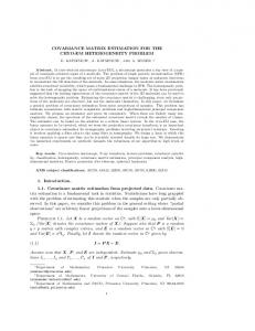
3 Experiment Settings In this work, the 32 textures used are from the Brodatz texture dataset [11]. This dataset were used in [7][12][13] and is shown in Figure 2. The entire Brodatz texture dataset is not used as the problem is harder to be solved for large number of classes with a limited sample size for each class respectively.

Fig. 2. 32 textures from the Brodatz texture dataset [12]

Each of the textures is separated into 16 partitions of size 64 × 64, each of the partition has four different variations, i.e. the original image, a rotated image, a scaled image and an image both rotated and scaled. Therefore there are a total of 16 sets for each texture with four samples in each set. For the training purpose, eight sets are randomly selected while the remaining eight sets are used for testing.

For the Gabor filters, a 31×31 filter was used with three radial center frequencies and eight orientations. The 24 Gabor filters are then used as the feature images to generate a 24 × 24 covariance matrix. All experiments were tested on ten different training and testing sets which are randomly chosen using the criteria as mentioned at the first paragraph of this section.

4 Results and Analysis Three different experiments are conducted. The first experiment is done by using intensity image and its edge-based derivative images as the feature images. The second experiment is done by using four different GLCM as the feature images. The last experiment is our proposed method of using Gabor filters as the feature images. 4.1 Experiment Result for Edge-based Derivative as Feature Images The first experiment uses the five feature image as proposed in [9] which includes the intensity image, first derivative with respect to x using [-1 2 -1]T filter, second derivative with respect to x, first derivative with respect to y using [-1 2 -1] filter and second derivative with respect to y. The feature images contain edge-based information on the vertical and horizontal directions. It generates a 5×5 covariance matrix. The accuracy achieved using this method is 84.65%. 4.2 Experiment Result for GLCM as Feature Images The second experiment uses four GLCMs as the feature images. The GLCMs are having spatial distance of one pixel and four orientations which are 0°, 45°, 90° and 135° [13]. It generates a 4 × 4 covariance matrix. The experiment is conducted for different numbers of grey level which are 8, 16, 32, 64, 128 and 256. The results are shown in Table 1 where the horizontal bar shows the number of grey level. Table 1. Recognition results for different numbers of grey level

(%) Accuracy

8 74.56

16 79.94

32 75.61

64 69.21

128 56.67

256 41.03

The best recognition rate is 79.94% for number of grey level of 16. When the number of grey level is high, the accuracy is very much lower. At a higher number of grey levels, the variance of the GLCM within samples of the same class can vary in a greater scale due compared to those with a lower number of grey levels since similar grey values are regarded as one at lower number of grey levels, reducing the variance within samples of the same class.

4.3 Experiment Result for Gabor Filters as Feature Images The last experiment uses the Gabor filters as the feature images for the covariance matrix. There are 3 radial center frequencies and 8 orientations used for the experiment, therefore having 24 feature images. It generates a 24 × 24 covariance matrix. Another experiment is done for only 4 orientations, therefore only generates a 12 × 12 covariance matrix. The results are shown in Table 2. Table 2. Recognition results for Gabor filters as feature images

(%) Accuracy

12 Gabor Filters 89.74

24 Gabor Filters 91.86

The best recognition rate is 91.86% for 24 Gabor filters. When fewer Gabor filters are used, the features are less and therefore the accuracy is slightly lower. The results are much better compared to the two previous experiments because the Gabor filters is able to extract frequency images in larger number that feeds in more information for the generation of covariance matrix compared to the previous techniques. 4.4 Analysis From the results that are obtained from this paper, we compared it with the recognition rates that are achieved in our previous works as shown in Table 3. Table 3. Comparison of recognition rates

(%) GLCM features Gabor features GLCM + Gabor features Raw GLCM Covariance Matrix (Edge-based Derivatives) Covariance Matrix (GLCM) Covariance Matrix (Gabor filters)

Accuracy 85.73 79.87 91.06 90.86 84.65 79.94 91.86

From the results, we can observe that Gabor filters are not powerful enough to discriminate textures to a high accuracy when it is working by itself, but when it is combined with other techniques; it helps to improve the accuracy. For the GLCM the accuracy is higher when it works independently but when it is used to generate a covariance matrix, feature are lost as the covariance matrix is only having the size of 4 × 4 with only 10 features. Therefore, the GLCM is not suitable to be used here.

5 Conclusion The results shows that the use of Gabor filters as the feature image for the covariance matrix is much useful than the use of edge-based derivatives or co-occurrence matrices as the feature image for the texture classification problem. The Gabor filters which are not performing as good when used independently can however produce a useful covariance matrix that can produce a better result.

6 Acknowledgement This research is partly funded by Malaysian MOSTI ScienceFund 01-02-11-SF0019.

References 1. Tuceryan, M., Jain, A.K. Texture analysis. In: The Handbook of Pattern Recognition and Computer Vision (2nd Edition). pp. 207-248. World Scientific Publishing, Singapore (1998) 2. Lew, Y.L.: Design of an Intelligent Wood Recognition System for the Classification of Tropical Wood Species. M. E. Thesis, Universiti Teknologi Malaysia (2005) 3. Tou, J.Y., Lau, P.Y., Tay, Y.H.: Computer Vision-based Wood Recognition System. In: Proc. Int’l Workshop on Advanced Image Technology. Bangkok (2007) 4. Partio, M., Cramariuc, B., Gabbouj, M., Visa, A.: Rock Texture Retrieval using Gray Level Co-occurrence Matrix. In: Proc. of 5th Nordic Signal Processing Symposium (2002) 5. Yap, W.H., Khalid, M., Yusof, R.: Face Verification with Gabor Representation and Support Vector Machines. In: IEEE Proc. of the First Asia International Conference on Modeling and Simulation (2007) 6. Chen, Y.Q. Novel techniques for image texture classification. PhD Thesis, University of Southampton, United Kingdom (1995) 7. Tou, J.Y., Tay, Y.H., Lau, P.Y.: Gabor Filters and Grey-level Co-occurrence Matrices in Texture Classification. In: MMU International Symposium on Information and Communications Technologies. Petaling Jaya (2007) 8. Nixon, M., Aguando, A.: Feature extraction and Image Processing. Butterworth-Heinemann, Great Britain (2002) 9. Tuzel, O., Porikli, F., Meer, P.: Region Covariance: A Fast Descriptor for Detection and Classification. In: European Conference on Computer Vision, 1, pp. 697-704 (2006) 10.Forstner, W., Moonen, B.: A Metric for Covariance Matrices. Technical report, Dept. of Geodesy and Geoinformatics, Stuttgart University (1999) 11.Brodatz, P.: Textures: A Photographic Album for Artists and Designers. Dover New York (1996) 12.Ojala, T, Pietikainen, M., Kyllonen, J.: Gray level Cooccurrence Histograms via Learning Vector Quantization. In: Proc. 11th Scandinavian Conference on Image Analysis, pp. 103108 (1999) 13.Tou, J.Y., Tay, Y.H., Lau, P.Y.: One-dimensional Grey-level Co-occurrence Matrices for Texture Classification. In: International Symposium on Information Technology. Kuala Lumpur, 3, pp. 1592-1597 (2008)