GDRouter: Interleaved Global Routing and Detailed Routing for Ultimate Routability Yanheng Zhang Placement Technology Group Cadence Design Systems San Jose, CA 95134 USA
[email protected] ABSTRACT Improving detailed routing routability is an important objective of a global router. In this paper, we propose GDRouter, an interleaved global routing and detailed routing algorithm for the ultimate routability i.e., detailed routing routability. The newly proposed router makes the global routing aware of detailed routing routability by correctly setting global capacity to reduce the inconsistency between the two stages. The final result contains both the detailed routing guided global routing and deailed routing solutions. Fast and efficient academic global routing and detailed routing tools FastRoute [1] and RegularRoute [2] are interleaved in GDRouter. In the Initial Capacity and Routing Weight Esitmation (ICRWE) phase, the weight for each global and detailed routing grid is calculated to make GDRouter aware of pin distribution based on a Gridded Voronoi Diagram method. Then the algorithm generates initial global capacity based on both local usage and global segment usage. In particular, Spine routing is utilized to estimate local usage. And a virtual routing i.e. fast implementations of FastRoute and RegularRoute, is performed to estimate global segment usage. The initial global capacity is applied in Full Routing phase to obtain detailed routing routability i.e., number of unassigned global segment. To further improve routability, in the following Iterative Test Routing (ITR) phase, GDRouter incrementally applies the interleaved global routing and detailed routing to adjust the global capcity based on detailed routing solution. To save runtime, GDRouter quits the loop if detailed routing routability stops improving or it reaches maximum iteration. Experimental results reveal that the newly proposed algorithm is capable of enhancing detailed routing routability. In particular, GDRouter reduces number of unassigned global segments by 90% for ISPD98 [3] derived testcases and around 60% for ISPD05/06 [4, 5] derived testcases with 2.9× runtime overhead.
Categories and Subject Descriptors B.7.2 [Hardware]: Integrated Circuits—Design Aids
General Terms Algorithms, Design, Performance
Keywords Routing, Physical Design, VLSI CAD
1.
INTRODUCTION
VLSI routing is an important design stage where module and cell pins are connected by over-the-cell metal wires. As the fabrication technology enters the nanometer scale, the routability issue is becoming increasingly challenging. First, there are more and more transistors integrated on chip and the size of routing problem is growing
Permission to make digital or hard copies of all or part of this work for personal or classroom use is granted without fee provided that copies are not made or distributed for profit or commercial advantage and that copies bear this notice and the full citation on the first page. To copy otherwise, to republish, to post on servers or to redistribute to lists, requires prior specific permission and/or a fee. DAC 2012, June 3-7,2012,San Francisco, California, USA. Copyright 2012 ACM 978-1-4503-1199-1/12/06 ...$10.00.
Chris Chu
Department of ECE Iowa State University Ames, IA 50010 USA
[email protected]
much bigger. Second, the integration of reusable unit of logic i.e., Intellectual Property (IP) cores due to the increasing design complexity poses more constraints on routing resources. It has been proved that the routing problem, even the small case containing only a couple of two-pin nets, is NP-hard [6]. Due to the enormous computational complexity, routing is typically carried out through consecutive global routing and detailed routing stages. In global routing, the entire routing region is divided into regular global cells(i.e., G-Cells) and routing is performed based on these G-Cells. The obtained global routing results are used to generate detailed routing solution considering exact metal shapes and positions.
Name adaptec1 adaptec2 adaptec3 adaptec4 adaptec5
FastRoute [1] O.F. CPU(sec.) 0 195 0 48 0 324 0 66 0 559
RegularRoute [2] unassiged CPU(sec.) 3233 566 1038 442 3352 1285 4027 1330 8826 3782
Table 1: Detailed routing results generated by RegularRoute on five reportedly routable global routing benchmarks in ISPD07/08 [7, 8] global routing contest The primary objective for global routing is to generate a congestion free global routing solution on G-Cells where the wiring demands across the G-Cell boundary is below its capacity. The global capacity is an estimation of how many wires can be accommodated during detailed routing. There have been many research conducted on improving global routing routability since the two consecutive ISPD 2007 and 2008 global routing contests [7, 8]. For instance, contestwinning routers like BoxRouter [9], NTHU-R [10], FGR [11] and FastRotue [1,12] are proposed to drive the global routing congestion lower with consistent effort. However, the ultimate routability i.e., detailed routing routability is not consistently pursued. In Table 1, we present the detailed routing results by taking the global routing solution of five routable testcases generated by the FasRoute. According to Table 1, all five testcases are easily routable by FastRoute in global routing stage. We use recently proposed detailed router RegularRoute [2] to generate the detailed routing solution. Nevertheless, none of the testcases can be easily routed by RegularRoute based on the pre-defined pitch size. The detailed routing routability i.e., number of unassigned global segment reaches several thousands. The results reveal the inconsistency between global routing and detailed routing stages. Or in other words, global capacity is not set in agreement with the detailed routing routability. Traditionally, global capacity is estimated based on empirical methods. For instance, to reserve routing resources for local usage and pin escape routing, global capacity is reduced for global edges on first horizontal and vertical metal layers. To simulate the effect of macro porosity for big macros, global capacity of the covered global edges is scaled by a fixed percentage. However, these methods are not accurate enough to estimate the detailed routing routability since they simply overlook the exact pin distribution and actual detailed routing usage. In this paper we will present a novel algorithm called GDRouter for the overall routability in routing problem. We intend to address the inconsistency between global and detailed routing by setting the global capacity more accurately. It is a systematic approach interleaving both global routing and detailed routing beyond the scope defined in conventional routing flow. As far as we know, it is the first attempt in academia to interleave the global routing and detailed routing for the detailed routing routability. Efficient global routing and detailed routing tools FastRoute [1] and RegularRoute [2] are interleaved. In the the Initial Capacity and Routing Weight Estimation (ICRWE) phase, we calculate the weight for each global and detailed routing grid to make GDRouter aware of pin
distribution. We propose a Gridded Voronoi Diagram method to eval- Segments uate pin distribution. We also generate initial global capacity based on local usage and global segment usage. In particular, we use a Spine routing technique to estimate the local usage. And we apply a virtual panel routing based on fast implementations of FastRoute and RegularRoute to estimate global segment usage. The initial global capacity is applied in the Full Routing phase to obtain detailed routing routability. In the following Iterative Test Routing phase, we run interleaved global routing and detailed routing to further improve routability. Detailed routing solutions are adaptively used to update global capacity. To speed up the whole algorithm, we propose incremental global routing Upper and a history based detailed routing for FastRoute and RegularRoute layer respectively. To save runtime, GDRouter terminates when it reaches maximum iteration or detailed routing routability stops improving. Therefore, the novel techniques that will be presented in this paper are as follows: • Novel routing algorithm interleaving global routing and detailed routing for detailed routing routability • Effective initial capacity and routing weight estimation capturing pin distribution, local usage and global segment usage • Efficient mechanism to adaptively update the global capacity based on detailed routing solutions • Useful incremental global routing technique and history based detailed routing technique to reduce runtime overhead We implemented GDRouter and tested its performance on routing testcases drived from ISPD98 [13] and ISPD05/06 [4, 5] benchmarks respectively. Experimental results show that GDRouter is capable of improving detailed routing routability in terms of number of unassigned global segments. In particular, the number is improved by 90% for ISPD98 and around 60% for ISPD05/06 with 2.9 × runtime overhead. The rest of the paper is organized as follows: In Section 2, we first review the global routing and detailed routing tools FastRoute and RegularRoute and present the overview of GDRouter. Section 3 discusses the initial capacity and routing weight estimation (ICRWE) phase. In Section 4, we present techniques in iterative test routing (ITR) phase for how to update global capacity based on detailed routing solution. Experimental results are presented in Section 5 and we will make conclusion of this paper in Section 6.
2.
GDROUTER OVERVIEW
In this section, we will first present necessary definitions and problem formulations for global routing and detailed routing respectively. We then present review for global and detailed routing tools FastRoute and RegularRoute. Finally, we will present the flow of GDRouter.
2.1
Problem Formulation
We will introduce the formulation for global routing and detailed routing respectively.
2.1.1
Global Routing Formulation
In global routing, layout region on each metal layer is divided into 3D global routing cells (3-D G-Cells). The 3-D global routing grid graph is drived where each grid denotes one 3-D G-Cell and each 3-D global edge represents the common boundary between two 3-D G-Cells. Each edge is assigned with 3-D global capacity representing the maximum allowable global routing usage. The overflow is the exceeding amount of global routing usage over global capacity. The major objective in global routing is to minimize total overflow. Since FastRoute generates 2-D global routing solution, we lump the 3-D G-Cells on different layers into a 2-D global routing cells (2-D G-Cell or simply G-Cell). The capacity, usage and overflow will be accumulated as the capacity, usage and overflow of the G-Cell respectively. The 3-D grid graph is therefore projected to become a 2-D grid graph. The global routing solution is generated using global path based on the 2-D grid graph. 1
2.1.2
Detailed Routing Formulation
The detailed routing resource is modeled as a 3-D regular grid graph. Each grid edge can accommodate exact one wire detailed routing usage. Please note that the grid defined here are not of the same concept with the global routing counterpart. We call the grid detailed routing grid or finest grid. It is defined by the pitch size so the detailed routing path on the grid would not cause spacing rule violations. Each routing layer has a preferred routing direction and the preferred direction iterates between adjacent layers. The routing track is defined as 1 In the following contexts, G-Cell, global edge and global capacity mean 2-D G-Cell, 2-D global edge and 2-D capacity.
track
3-D global edge
G-Cell
via
(b)
(a)
Figure 1: Problem formulation for global routing and detailed routing (a) Detailed routing with panel, track, segments with two layers (b) Corresponding global routing grid graph Input 2-D Global Routing Solution and 3-D Grids Local Nets Routing by Single Trunk V-Tree Track Routing
Global Segment Extraction Pin
Global Segment Assignment Unassigned segments Assigned segments
Output Detailed Routing Solution
via
Regular Routing
(a)
(b)
Figure 2: (a) Overview of RegularRoute (b) Comparison between track routing and regular routing a sequence of grid edges along the preferred routing direction of each layer. The input is 2-D global routing solution We extract global segments from the global routing solution. Each global segment spans multiple G-Cells that the global route goes through. Panel is defined to be the collection of parallel tracks in a row of column of G-Cells for each metal layer. It is introduced to favor the global segment assignment for paralleism. Spacing rule related design rule violations account for the majority of design rule violations in a typical VLSI design. We mainly consider the spacing rules during detailed routing since they have been captured by the application of detailed routing grid. The congestion of detailed routing is evaluated by the number of unassigned global segments, meaning such global segments cannot be properly assigned due to conflicts with other usage. In Figure 1, we show the definitions we have mentioned for global routing and detailed routing respectively. Simply speaking, global routing generates global routing solution based on 2-D global routing grid. The obtained results are used to generate the detailed routing solution based on detailed routing grid. Hence the ultimate routability should be pertinent to the congestion (number of unassigned segments) of detailed routing solution.
2.2
FastRoute and RegularRoute
Next we introduce the global routing and detailed routing algorithms that are interleaved in GDRouter. FastRoute is very fast and effective global router. It incorporates a couple of ideas for solving the challenging global routing testcases. It contains a number of works: FastRoute [14] is the first work which presented congestion-driven Steiner tree construction and edge shifting. FastRoute 2.0 [15] introduced a novel monotonic routing to enhance the pattern routing and a multi-source multi-sink maze routing to improve maze routing. In FastRoute 3.0 [12], a virtual capacity technique is proposed to achieve fast convergence of maze routing. FastRoute [1] introduces routing techniques for reducing via count. RegularRoute [2] is a recently proposed grid-based detailed routing technique. The router strives to generate regular routing patterns (less turning) to benefit design rule satisfaction. In general, it adopts a bottom-up layer-by-layer and panel-by-panel scheme. It employs a spine routing technique to route the local nets. The global segments are assigned panel-by-panel and a Maximum Weighted Independent
Set (MWIS) problem is formulated for each panel. RegularRoute employes a fast and effective heuristic to solve the problem for each panel. For better detailed routing routability, the router introduces the terminal promotion and partial assignment. RegularRoute looks similar to the track routing problem [16] but there are great difference between the two. One important factor is that RegularRoute generates a valid detailed routing solution where terminal connections are considered. General track routing simply overlooks terminal connection. In Figure 2(a), we show the overview of RegularRoute and its algorithmic flow. In Figure 2(b), we present the example of solutions for both RegularRoute and general track routing. We could easily discover the difference between the two problems.
2.3
Algorithm Flow
The general flow of GDRouter is shown in Figure 3. Basically the flow contains three main phases: (1) Initial Capacity and Rouing Weight Estimation (2) Full Routing (3) Iterative Test Routing. The flow of GDRouter interleaves the flow of FastRoute and RegularRoute but it is not simply an addition of the two. There are many new techniques introduced for better detailed routing routability and less runtime overhead. Phase 1: Initial Capacity and Routing Weight Estimation 1. Pin distribution analysis based on Gridded Voronoi Diagram of detailed routing grids 2. Local usage estimated by Spine routing 3. Virtual routing by fast implementations of FastRoute and RegularRoute Phase 2: Full Routing 4. FastRoute 5. Global segment extraction 6. RegularRoute Phase 3: Iterative Test Routing 7. Global capacity update based on RegularRoute’s solution 8. Incremental FastRoute to reroute nets with unassigned global segments 9. History based RegularRoute to tune number of choice of global segments 10. Repeat Phase 3 until reaching maximum iteration or detailed routing routability stops improving
Figure 3: Flow of GDRouter In particular, in ICRWE phase, pin distribution is analyzed based on Gridded Voronoi Diagram. The weight for each global and detailed routing grid is calculated and will be applied in the following global and detailed routing. Spine routing and a virtual routing are performed to generate the initial global capacity based on the estimated local usage and global segment usage. Based on the initial global capacity computed in Phase 1. GDRouer applies FastRoute and RegularRoute in full-routing mode to obtain detailed routing soluiton. Next, GDRouter enters routing (ITR) phase to iteratively update the global capacity to make sure the global routing is guided to avoid detailed routing hotspots. To speed up the whole algorithm, an incremental global routing technique and a history based global segment assignment technique are applied for FastRoute and RegularRoute. They are proposed to replace the time-consuming full routing. It should be noted that in GDRouter, detailed routing has been fully integrated in our full-chip routing framework. The final routing solution contains not only the detailed routing guided global routing solution, but also the very detailed routing solution accompanied with it.
3.
INITIAL CAPACITY AND ROUTING WEIGHT ESTIMATION
In this section, we will introduce techniques in ICRWE phase in detail. In the first part, we will discuss a Gridded Voronoi Diagram method to analyze pin distribution and how to compute the weight for each global routing and detailed routing grid. Next, we introduce the Spine routing to estimate local usage. Finally, we discuss virtual routing to capture the global segment usage by fast implementations of FastRoute and RegularRoute and how we generate initial global capacity based the two techniques.
3.1
Pin Distribution Analysis based on Gridded Voronoi Diagram
Pin distribution is an important indicator of potential routing congestion. In the past, people usually use pin density i.e., number of pins in one G-Cell to estimate pin related local hotspots. However, pin density cannot fully capture detailed routing routability. Consider one G-Cell containing 5 pins with even distribution while the other G-Cell with 4 pins but with all pins concentrated in the G-Cell. The latter one has lower pin density but more likely to be unroutable.
4
Seed A
3
P
a
b
2
Q
B
M C
1
0 0
1
2
3
4
(b)
(a)
Figure 4: (a) General Voronoi diagram with seeds and proximity cells (b) Gridded Voronoi Diagram of detailed routing grid Therefore we propose to adopt pin distribution analysis along with pin density in GDRouter. In the work of [17], the paper utilizes voronoi diagram [18] to estimate the wire distribution and the corresponding critical area. In this paper, we utilize Gridded Voronoi Diagram to estimate pin distribution. In a general Voronoi Diagram, the entire region indicates the whole area under analysis, a seed indicates the subject of which we are investigating the distribution (e.g., pin in our case). The proximity cell of a seed is the sub-region in which each point has closest proximity to the seed. The proximity cell boundary consists of the points along the cell boundary, which have equivalent cloest proximity to multiple seeds. Figure 4 illustrates a general voronoi diagram for a region with nine seeds. For instance, point a belongs to seed P , and point b is along the cell boundary of seed Q and has equal proximity to P and Q. The size of proximity cell indicates the distribution in the area around the particular seed. For the case with evenly distributed seeds, the voronoi diagram proximity cell is equivalent in size. For a case with non-evenly distributed seeds, the relative size of the proximity cell indicates the seeds’ distribution i.e., the smaller the size of a cell, the denser seed’s distribution will be. For instance, in Figure 4(a), seed P has smaller proximity cell than seed M , so points around P have denser seeds’ distribution than M . Based on this intuition, we could extend the general voronoi diagram to detailed routing grid, and we call it Gridded Voronoi Diagram. The main difference is the the region is now grid based and the seed has become the pin. In our formulation, since each pin is located on one detailed routing grid of M1 (metal 1), we will only look at the 2-D detailed routing grid in M1 instead of other metal layers. We define the proximity grids for a pin as the detailed routing grids with closest proximity to a pin. And we define the peripheral grids as the grids with equivalent cloest proximity with multiple pins. To analyze the pin distribution for each grid, we first calculate the average count of proximity grids (θ) for all pins, which is equal to total grids divided by total pins. For any pin, we supppose the pin has g proximity grids, the distribution for the pin’s proximity grids is calculated as follows, θ Dgpx = β × ( )α g θ × (p + 1) β= W2
(1) (2)
where α is a parameters that need be tuned for optimization. In our experiemnt, alpha equals 1.5. β is another factor tuning the distribution value. W is the length of square window which contains number of grids cloest to g i.e., W 2 ≈ g . p is the number of pins inside the window.2 For each peripheral grid, its distribution is equal to the average of all pins it has closest proximity. P px Dg Dgpr = (3) Npr In the equation Npr is the total number of pins the peripheral grid has closest proximity. A gridded voronoi diagram for detailed routing grids is illustrated in Figure 4, which contains a 5×5 grid with three pins. We list out the closest proximity pin for each grid. For instance, grid (1, 1) in coordinate is a peripheral grid which has equivalent closest proximity to pin B and pin C. While grid (2, 0) and (2, 1)are two proximity grids of pin C. And the pin distribution for each grid can ben computed accordingly. 2 The window is introduced to partly capture the impact of pin density and to defferentiate grids in the same proximity cell.
The pin distribution of one G-Cell is calculated by averaging all grids inside the G-Cell including both proximity grids and peripheral grids, which is P Dg Dcell = (4) G In the equation, Dcell is the average pin distribution value of G-Cell, and G is the number of grids inside the G-Cell. Based on these computations, we assign the weight of each G-Cell in global routing and each detailed routing grid in detailed routing. More specifically, in global routing, the global path generation is weighed by Dcell . And during detailed routing, the cost of assigning each global segment is also weighed by Dg .
3.2
Local Usage Estimation
One factor that may affect global capacity is the local usage inside one G-Cell. A net or part of a net that resides inside a G-Cell is a local net. The local usage is treated as blockages when assigning global segments. Hence global capacity needs to be adjusted. In RegularRoute, spine routing is applied to route local nets. Spine routing construct routing tree using one vertical trunk and several horizontal branches. The major advantage in terms of routability is the preservation of routing resources. We apply spine routing for estimating local usage.
shapes [19]. Although we may not obtain overflow free global routing solution, it provides with the information of global segment usage with actual global routing paths. Next, the global routing solutions are imported into RegularRoute. Likewise, we employ a fast mode of RegularRoute with restricted solution space instead of trying to generate the optimized solution. In particular, each global segment is allowed to try fewer regular routing shapes. Terminal promotion and partial assignment are disabled for saving runtime. As a matter of fact, in such configuration, we only perform track routing. After virtual routing, we obtain the detailed routing routability in terms of the unassigned global segments. For each global edge e along the unassigned global segment, suppose we have the global capacity Ce , the global routing overflow Oe and the total number of unassigned segments is Ue . Although global edge e has global routing overflow Oe , in detailed routing, the actual unassigned global segment is Ue . The mismatch of global capacity and detailed routing is actually Ue − Oe . We adjust the global capacity by the following equation, Ce′ is the new capacity, γ is a coefficient to suppress the over-adjustment of the global capacity. γ equals 0.5 in our experiment. Ce′ = Ce − γ × (Ue − Oe )
(5)
Based on the spine routing and the virtual routing, we obtain the inital global capacity. With the initial global capacity, GDRouter enters full routing phase in which FastRoute and RegularRoute are applied in full-routing modes.
G-Cell
4. Close to Boundary -1 Exceed track limit -1
-1
ok
Figure 5: (a) Spine routing for estimating local usage We reduce the global capacity for a global edge if local usage is close to the boundary of the G-Cell (smaller than 3 grids) or the total usage of one track inside the G-Cell is over 50%. Local usage that close to GCell boundary is likely to block global segment usage (routing across the G-Cell). And the track is likely to be blocked when the total local usage is high, in which case we need to reduce capacity for both global edges (e.g., left and right edges). In Figure 5, we show global capacity adjustment when local usage is close to G-Cell boundary. It is also illustrated that one track is assigned with usage more than 50%, the capacity is reduced for both left and right global edges.
3.3
Virtual Routing for Estimating Global Segment Usage
The mere local usage estimation is not capable of accurately finding detailed routing hotspots. In many cases, congestion occurs simply when global segment cannot be assigned. In Figure 6, we show a congested global edge with the global capacity of four. And the global edge is used by four nets, which does not cause overflow in global routing. But in reality only three of the segments can be assigned in detailed routing. In this case congestion is caused by global segment usage and the mismatch between global capacity and detailed routing routability. Since it is computationally hard to predict global segment usage and its impact on global capacity, we propose to apply a virtual routing for global capacity adjustment. The virtual routing consists of fast implementations of global and detailed routing. In particular, in FastRoute, we only apply very fast pattern routing in ”L” and ”Z”
Global Edge C_e = 4 U_e = 1 O_e = 0
G-Cell
Figure 6: Global segment derived congestion in detailed routing without pin and local usage
ITERATIVE TEST ROUTING
In this section we present techniques in the iterative test routing (ITR) phase. The main idea is to update global capacity iteratively based on interleaved global and detailed routing. Detailed routing routability in terms of unassigned global segments is utilized to adjust the global capacity. To improve runtime, an incremental global routing technique is proposed for the interleaved global routing. And a novel history based detailed routing technique is proposed for the interleaved detailed routing. ITR terminates when it reaches maximum iteration or the number of unassigned global segments stops improving. In the end, the routing solution contains not only a detailed routing guided global routing solution, but also the very detailed routing solution accompanied with it.
4.1
Adaptive Global Capacity Update
4.2
Techniques to Reduce Runtime Overhead
As the flow shown in Figure 3, after ICRWE, we apply global routing and detailed routing using FastRoute and RegularRoute with fullrouting features. During the global routing stage, the 2-D global routing solution in terms of the global route on the global routing grids is obtained. We extract global segments based on the solution. In the subsequent detailed routing stage, RegularRoute is applied to route local nets and assign global segments. After detailed routing, the detailed routing routability is obtained in terms of the number of unassigned global segments, with the indication of where the actual detailed routing congestion is. We need to update the global capacity to make sure global routing is properly guided by actual detailed routing bottlenecks. As defined in Section 2.1.2, a global segment represents an interval spanning multiple G-Cells. It should be assigned to the tracks to the panels it belongs to. If a segment is unassigned, it suggests the panels are unable to accommodate the segment. We update global capacity based on the global edges along the unassigned global segment. For each global edge e after detailed routing, Ae is the number of assigned global segment, Ce is the original global capacity, Ue is the number of unassigned segments, and Re is the accumulated amount of capacity adjustment (positive for reduction, negative for increase). We will adaptively update the global capacity based on the following cases (we use Ce′ to represent the new capacity): i) If Ae + Ue > Ce + Re and Ue > 0.2 × (Ce + Re , when the global capacity is excessively overestimated, Ce′ = Ce × 0.9; ii) If Ae + Ue > Ce + Re and 0.2 × (Ce +Re ) ≥ Ue > 0, when global capacity is moderately undertimated, Ce′ = Ce − 1; iii) If Ae + Ue ≤ Ce + Re − 2 and Ue = 0, when global capacity is underestimated, Ce′ = Ce + 1; iv) In all other cases, when global capacity is roughly accurate, Ce′ = Ce . In general, capacity reduction and increase is carried out without too large amount since (1) The detailed routing hotspot may change over-time, it is not proper to drastically reduce the global capacity. (2) We do not intend to disturb the original solution, otherwise it takes more computational effort in the subsequent global routing and detailed routing in ITR. Runtime is the major overhead in ITR if we apply FastRoute and RegularRoute in full-routing features. As a matter of fact, in very congested designs global capacity might become very restricted, and the global routing could become too congested to achieve routing convergence. In such case, RegularRoute would spend longer runtime due to
the extra global segment usage introduced by the detoured global path in FastRoute. To reduce runtime overhead, we propose techniques for FastRoute and RegularRoute to improve runtime in ITR. More specifically, we propose incremental global routing technique for FastRoute and history based global segment assignment for RegularRoute.
4.2.1
Incremental Global Routing
Instead of applying FastRoute with full features in ITR, we propose an incremental global routing technique. As introduced in Section 2.2, FastRoute is a sequential global router which is rip-up and reroute based. Nets are routed sequentially from step to step. Therefore, we rip-up and reroute nets using over-capacity edges. This approach would reduce the number of routed nets significantly. Moreover, most global routers like FastRoute strive to minimize global routing overflow and spend long runtime on maze routing. We propose to terminate maze routing when the congestion improvement is less than a threshold value, which is 5% of the initial total global routing overflow. After obtaining incremental global routing solution, we only re-extract the global segments of the nets that are rerouted.
4.2.2
History Based Detailed Routing
In RegularRoute, solution space of assigning global segment is explored based on a number of regular routing shapes i.e., the specific track, layer and terminal routing, of each global segment. Each candidate shape is defined as one Choice of the segment. Basically one segment is more flexible given more choices. As noted earlier, to perform RegularRoute in full features inside ITR would be very computationally expensive. We propose the history based detailed routing to reduce runtime overhead. In particular, for the nets that are not rerouted in incremental global routing, we will recommend to use the choices of global segments of last iteration, or in other words, we rank the recommended those choices with higher priority. If one segment is consistently assignable, we gradually decrease the number of choice or even just provide the choice of last iteration. This technique is especially effecitve for the panels that are not congested. Conversely, for the tough-to-handle global segments, we increase their number of choices to improve routability. But with the algorithm continues, fewer global segments are unassignable and the runtime for each iteration of ITR is further reduced.
5.
EXPERIMENTAL RESULTS
We implement GDRouter in C and all our experiments are performed on a machine with 2.67GHz Intel Xeon CPU and 32G memory. We derive the testcases from ISPD98 [3] and ISPD05/06 [4, 5] placement benchmarks. In original ISPD98 benchmarks, pins are set to be at the center of each standard cell, we develop a program to randomly set the pin coordinates and make sure they satisfy the spacing requirements at the bottom layer.3 We use Dragon [20] to generate the placed testcases for ISPD98 benchmarks and use FastPlace [21] to generate those for ISPD05/06 benchmarks. Other placement methods [22] [23] [24] are worthy alternatives but it is out of the content of this paper. We will then derive the global routing benchmark based on placed testcase with the same format as ISPD07/08 global routing contest benchmarks [7, 8].
5.1
Initial Capacity Estimation Results EM1 EM2 EM3 ICRWE Name unass- CPU unass- CPU unass- CPU unass- CPU igned (sec.) igned (sec.) igned (sec.) igned (sec.) ibm01 0 9.7 0 7.3 4 18.6 0 11.2 ibm02 25 19.2 36 15.6 78 44.3 21 18.4 ibm07 55 37.6 66 34.3 108 98.5 43 42.5 ibm08 19 62.4 23 41.6 26 122.1 20 57.1 ibm09 24 78.2 32 52.5 42 175.2 19 55.4 ibm10 55 98.4 65 73.2 99 188.4 34 103.6 ibm11 25 93.4 19 68.9 46 155.9 16 87.2 ibm12 145 206.5 168 114.5 255 355.2 102 137.2 Sum 348 605.4 409 407.9 658 1158.2 255 512.6 Norm 1.36 1.48 1.60 1 2.58 2.84 1 1.26
Table 2: Results comparison with three empirical methods for estimating global capacity up to full routing phase (Phase 2) in GDRouter on ISPD98 derived testcases. We present experimental results of techniques in the initial capacity and routing weight estimation phase on ISPD98 derived testcases. The results are summarized in Table 2. We compare ICRWE against three empirical methods, namely EM1, EM2 and EM3 respectively. In particular, EM1 assumes the first two metal layers (M1 and M2) have 3
We assume all pins are on M1.
0% of full capacity and the rest of layers have 50% of the full capacity. EM2 assumes the first two metal layers have 20% of full capacity and the rest of layers have 80%. And EM3 assumes the first two metal layers have 40% of full capacity and the rest of layers have 100%. In our experiments, all parameters are identical for the four cases. In Table 2, we present the results for each case respectively. We could notice that ICRWE is capable of achieving best routability among the four methods. EM1 tends to underestimate the global capacity. It makes the global routing much harder to solve and creates more extra detours. The extra detoured usage is likely to incur more global segment usage and thus affect detailed routing routability. On the other hand, EM3 tends to overestimate the global capacity. The global routing problem in EM3 is easier to solve, but it leads to a harder-to-solve detailed routing problem. The runtime becomes much worse since the runtime spent on detailed routing increases dramatically. EM2 generates reasonably good solution. But the same success cannot be guaranteed for all design cases. Overall, ICRWE provides more accurate global capacity estimation than the empiricle methods and it generates best routability.
5.2
GDRouter Results on ISPD98 Derived Testcases
We present experimental results for GDRouter on the eight ISPD98 derived testcases. We compare our results with three variations of GDRouter. All the results are summarized in Table 3. In the table, the first three columns provides us the basic statistics of the testcases. #N ets is the total number of nets in the testcase, Grid is the scale of global routing grid, Avg.Deg. is the average net degree for the entire netlist. These statistics provide an overview of the complexity for each testcase. The next columns show the results on three different variations of GDRouter. In particular, the first one is GDRouter without ICRWE phase. It applies EM2 (20% M1-M2, 80% All other layers). Second variation is GDRouer without ITR phase. It is the same as reported in Table 2 for the ”ICRWE” case. The third variation is GDRouter without incremental global routing and history based detailed routing techniques. And the last three columns show results for GDRouter with all proposed techniques. From the table, it is noticeable that all proposed techniques are indispensable in GDRouter. In particular, ICRWE provides a good starting point with more accurate initial global capacity. Likewise, ITR is an important component since the number of unassigned segments is consistently reduced in this phase. And the incremental global routing technique and history based detailed routing technique significantly reduce runtime overhead (roughly 2 times), though FastRoute and RegularRoute in full features generate slightly better QoR. In terms of runtime, GDRouer without ITR is close to conventional routing flow (except some runtime spent in ICRWE phase). It shows GDRouter is capable of reducing number of unassigned segments by 90% with 2.9× runtime overhead.
5.3
GDRouter Results on ISPD05/06 Derived Testcases
We present experimental results for GDRouter on the eight ISPD05 /06 derived testcases. Similarlly, we compare our results with three variations of GDRouter. All the results are summarized in Table 4. The circuit statistics report the similar metrics of each testcase. They are typically much larger in design size than the testcases derived from ISPD98 benchmarks. In ISPD07/08 [7, 8] global routing contests, the pitch size is set to 2 to make the global routing benchmarks more challenging. They are not easy to handle in detailed routing. Hence we perform our experiments on testcases with two cases (pitch size equals one and two respectively). Like the experiments on ISPD98 derived testcases, we compare GDRouter with three variations, GDRouter without ICRWE, GDRouter without ITR and GDRouter without incremental global routing and history based detailed routing. We could notice for large designs, GDRouter is also effective in improving detailed routing routability. In particular, it shows that GDRouter reduces over 60% unassigned global segments when pitch size is two and over 90% when pitch size is one. And it is also noticeable that all techniques are indispensable in GDRouter. In terms of runtime, GDRouter spends 2.8× and 2.1× of conventional routing flow (GDRouter without ITR) for the two cases with pitch size equals 2 and 1 respectively. Overall, GDRouter is capable of generating cost efficient detailed routing results.
6.
CONCLUSION
In this paper, we propose GDRouter: an interleaved global routing and detailed routing algorithm for the ultimate routability. It contains three phases: initial capacity and routing weight estimation (ICRWE), full routing and iterative test routing (ITR). Pin distribution is analyzed based on the novel Gridded Voronoi Diagram and each global grid and detailed routing grid is assigned weight based on
statistics Name ibm01 ibm02 ibm07 ibm08 ibm09 ibm10 ibm11 ibm12 Sum Norm
#Nets 11507 18427 44394 47944 50393 64227 66994 67739 -
Grid 133×132 152×151 229×228 239×238 243×242 316×315 276×275 341×340 -
Avg. Deg. 3.85 4.23 3.70 4.13 3.73 4.19 3.54 4.34 -
w/o ICRWE unassCPU igned (sec.) iter 0 7.3 0 2 54.6 5 0 104.2 4 0 130.9 4 8 162.3 4 6 221.6 5 8 213.6 4 30 466.7 7 54 1361.2 2.3 0.93 -
unassigned 0 21 43 20 19 34 16 102 255 11.1
w/o ITR CPU (sec.) 11.2 18.4 42.5 57.1 55.4 103.6 87.2 137.2 512.6 0.35
iter. 0 0 0 0 0 0 0 0 -
w/o unassigned 0 0 0 0 0 0 0 12 12 0.5
Runtime CPU (sec.) iter. 11.2 0 95.5 5 202.3 4 288.6 4 302.6 5 523.2 5 402.6 4 988.1 7 2814.1 1.9 -
unassigned 0 0 0 0 0 2 0 21 23 1
GDRouter CPU (sec.) 11.2 60.5 111.4 142.0 177.6 220.4 235.1 498.5 1456.7 1
iter. 0 5 4 4 5 5 4 7 -
Table 3: Results comparison for GDRouter for variations (GDRouter w/o ICRWE, GDRouter w/o ITR, GDRouter w/o incremental global routing and history based detailed routing in ITR) on ISPD98 derived testcases statistics Name adaptec1 adaptec2 adaptec3 adaptec4 adaptec5 newblue1 newblue5 newblue6 Sum Norm adaptec1 adaptec2 adaptec3 adaptec4 adaptec5 newblue1 newblue5 newblue6 Sum Norm
#Nets 219243 257659 466293 515300 867344 331106 1257334 1286448 / / / / / / / / -
Grid 893×892 1174×1172 1935×1946 1933×1945 1935×1946 934×932 2122×2132 2310×2318 / / / / / / / / -
Avg. Deg. 4.28 4.09 4.01 3.70 3.99 3.68 3.87 4.09 / / / / / / / / -
Pitch
2
1
w/o ICRWE unass- CPU igned (min.)iter 1244 42 4 221 24 3 1462 85 5 1755 67 4 3345 205 5 45 18 4 2821 197 5 3672 220 5 14565 858 1.09 0.96 0 12 0 0 8 0 2 42 2 0 48 3 30 155 4 0 5 0 24 139 4 16 98 3 72 507 3.27 0.95 -
w/o ITR unass- CPU igned (min.)iter. 3019 16 0 972 11 0 3177 29 0 3822 27 0 8467 74 0 376 7 0 7718 71 0 8892 84 0 36443 319 2.7 0.36 0 14 0 0 10 0 16 26 0 44 23 0 156 62 0 0 6 0 81 55 0 42 63 0 339 259 15.4 0.49 -
w/o Runtime unass- CPU igned (min.)iter. 1044 81 4 189 55 3 993 186 5 1450 110 4 2844 420 5 32 31 4 2444 409 5 3012 449 5 12008 1741 0.90 1.95 0 14 0 0 10 0 0 94 2 0 90 3 10 298 4 0 6 0 0 266 4 0 212 3 10 990 0.45 1.86 -
GDRouter unass- CPU igned (min.)iter. 1259 44 4 198 26 3 1088 89 5 1562 71 4 3177 211 5 34 19 4 2593 206 5 3411 226 5 13322 892 1 1 0 14 0 0 10 0 0 45 2 0 52 3 18 160 4 0 6 0 4 144 4 0 102 3 22 533 1 1 -
Table 4: Results comparison for GDRouter for variations on ISPD05/06 derived testcases pin distribution. Spine routing and virtual routing are applied to generate initial global capacity. In ITR, GDRouter further polishes the initial global capacity based on detailed routing results. Experimental results on both ISPD98 and ISPD05/06 derived testcases demonstrate the effectiveness and efficiency of our algorithm. We will continue to improve GDRouter’s performance and scalability. We will propose more systematic frameworks to perform capacity update. Meanwhile, we will also enhance the solution quality of the interleaved global routing and detailed routing algorithms.
7.
REFERENCES
[1] Y.Xu, Y.Zhang, and C.Chu. FastRoute 4.0: Global router with efficient via minimization. In Proc. Asia and South Pacific Design Automation Conf., pages 576–581, 2009. [2] Y. Zhang and C. Chu. RegularRoute: An efficient detailed router with regular routing patterns. In Proc. ACM/SIGDA Intl. Symp. on Physical Design, pages 146–151, 2011. [3] ISPD98 global routing benchmarks. http://www.ece.ucsb.edu/∼kastner/labyrinth. [4] ISPD05 placement contest benchmarks. http://www.sigda.org/ispd2005/contest.htm. [5] ISPD06 placement contest benchmarks. http://www.sigda.org/ispd2006/contest.htm. [6] M. R. Garey and D. S. Johnson. Computers and Intractability: A Guide to the Theory of NP-Completeness. Freeman, NY, 1979. [7] ISPD07 global routing contest benchmarks. http://www.sigda.org/ispd2007/contest.htm. [8] ISPD08 global routing contest benchmarks. http://www.sigda.org/ispd2008/contest.htm. [9] K. Yuan M. Cho, K. Lu and D. Z. Pan. Boxrouter 2.0: Architecture and implementation of a hybrid and robust global router. In Proc. Intl. Conf. on Computer-Aided Design, pages 503–508, 2007. [10] P.-C. Wu J.-R. Gao and T.-C. Wang. A new global router for modern designs. In Proc. Asia and South Pacific Design Automation Conf., pages 232–237, 2008. [11] M. M. Ozdal and M. D.F. Wong. High-performance routing at the nanometer scale. In Proc. Intl. Conf. on Computer-Aided Design, pages 496–502, 2007.
[12] Y. Zhang, Y. Xu, and C. Chu. FastRoute 3.0: A fast and high quality global router based on virtual capacity. In Proc. Intl. Conf. on Computer-Aided Design, pages 344–349, 2008. [13] IBM-Place 1.0 benchmark suites. http://er.cs.ucla.edu/benchmarks/ibm-place/. [14] M. Pan and C. Chu. Fastroute: A step to integrate global routing into placement. In Proc. Intl. Conf. on Computer-Aided Design, pages 464–471, 2006. [15] M.Pan and C.Chu. FastRoute 2.0: A high-quality and efficient global router. In Proc. Asia and South Pacific Design Automation Conf., pages 250–255, 2007. [16] S. Batterywala, N. Shenoy, W. Nicholls, and H. Zhou. Track assignment: A desirable intermediate step between global routing and detailed routing. In Proc. Intl. Conf. on Computer-Aided Design, pages 59–66, 2002. [17] H. Chen, S. Chou, S. Wang, and Y. Chang. Novel wire density driven full-chip routing for cmp variation control. In Proc. Intl. Conf. on Computer-Aided Design, pages 831–838, 2007. [18] M. de Berg, M. van Kreveld, M. Overmars, and O. Schwarzkoph. Computational Geometry: Algorithms and Applications. Springer, 1997. [19] E. Bozorgzadeh R. Kastner and M. Sarrafzadeh. Pattern routing: Use and theory for increasing predictability and avoiding coupling. IEEE Trans. on Computer-Aided Design and Integrated Circuits and Systems, 21(7):777–790, July 2002. [20] X.Yang, B.Choi, and M.Sarrafzadeh. Routability-driven white space allocation for fixed-die standard-cell placement. IEEE Trans. on Computer-Aided Design and Integrated Circuits and Systems, 22(4):410–419, April 2003. [21] N.Viswanathan, M.Pan, and C.Chu. FastPlace 3.0: A fast multilevel quadratic placement algorithm with placement congestion control. In Proc. Asia and South Pacific Design Automation Conf., pages 135–140, 2007. [22] Y. Zhang and C. Chu. CROP: Fast and effective congestion refinement of placement. In Proc. Intl. Conf. on Computer-Aided Design, pages 344–350, 2009. [23] J.Z. Yan and C. Chu. Handling complexities in modern large-scale mixed-size placement. In Proc. ACM/IEEE Design Automation Conf., pages 436–441, 2009. [24] J.Z. Yan and C. Chu. DeFer: defered decision making enabled fixed-outline floorplanner. In Proc. ACM/IEEE Design Automation Conf., pages 161–166, 2008.