Genetic Algorithms with Nelder-Mead Optimization in the ... - CiteSeerX

WSEAS TRANSACTIONS on MATHEMATICS

Nikos E. Mastorakis

Genetic Algorithms with Nelder-Mead Optimization in the variational methods of Boundary Value Problems NIKOS E. MASTORAKIS WSEAS Research Department Agiou Ioannou Theologou 17-23 Zografou, 15773, Athens, GREECE and Technical University of Sofia, English Language Faculty Industrial Engineering Department Sofia 1000, BULGARIA [email protected] and with the Military Institutes of University Education (ASEI), Hellenic Naval Academy, Terma Hatzikyriakou, Piraeus, GREECE

Abstract: - The p-Laplacian equation is a generalization of the PDE of Laplace Equation and in this paper, we present a way of its solution using Finite Elements. Our method of Finite Elements leads to an Optimization Problem that can be solved by an appropriate combination of Genetic Algorithms and Nelder-Mead . Our method is illustrated by a numerical example. Other methods for the solution of other equations that contain the p-Laplacian operator are also discussed. Keywords: - Boundary Value Problems, Finite Elements, Genetic Algorithms with Nelder-Mead. p-Laplacian, non-Newtonian fluid flow.

1 Introduction The combined method of Genetic Algorithms and Nelder-Mead was proposed by the author in 2005, [2]÷[9] , while the author proposed the solution of ODEs and PDES since July 1996 (See[1])).

operator), where the p-Laplacian operator is defined as follows p −2 Δ p u := div⎛⎜ ∇u ∇u ⎞⎟ ⎝ ⎠

problems in physics and mechanics are formulated in equations that contain the p-Laplacian, (i.e. the p-Laplace

G. Bognar in [17, presented a very interesting numerical and analytic investigation of

Many

nonlinear

ISSN: 1109-2769

107

Issue 3, Volume 8, March 2009

WSEAS TRANSACTIONS on MATHEMATICS

Nikos E. Mastorakis

∂u p−2 = div⎛⎜ ∇u ∇u ⎞⎟ + λu q , (4) ⎝ ⎠ ∂t where p > 1, q > 0 and λ are some constants,

problems of fluid mechanics that are described with PDEs containing the p-Laplacian operator. Previous publications (also reported in [17]) include reaction-diffusion problems, nonNewtonian fluid flows [18], fluid flows through certain types of porous media ([19], [20], the Lane-Emden equations for equilibrium configurations of spherically symmetric gaseous stellar objects [21], singular solutions for the Emden-Fowler equation [22] and the EinsteinYang-Mills equations [23], the existence and nonexistence of black hole solutions, nonlinear elasticity [24], glaciology [25] and petroleum extraction [26]. It is clear that for p = 2 :

in which the nonlinear term λu q describes the nonlinear source in the diffusion process, called "heat source" if λ > 0 and "cold source" if λ < 0. Just as the Newtonian equation ( p = 2), the appearance of nonlinear sources will exert a great influence to the properties of solutions and the influence of "heat source" and "cold source" is completely different. In [31], an attempt is made by the author to solve the equations (2), (3) and (4) using various numerical schemes. In this paper we will solve the boundary value problem

Δ p = Δ . The study of the p -Laplacian equation started more than thirty years ago. In recent years, rapid development has been achieved for the study of equation involving operator Δ p and a vast literature has appeared

(

div ∇u

The Problem is reduced to an Optimization problem that can be solved by Genetic Algorithms with Nelder-Mead. An early paper of the author with the title “Solving Differential Equations via Genetic Algorithms” was presented in [1]. Actually, the author presented in 1996 the solution of ODE and PDE using Genetic Algorithms optimization, while the author use the same method to solve various problems in [2]÷[9]. The main Results are given in Section 2 and a numerical example illustrates the method in Section 3. A discussion for the numerical solution of (2), (3) and (4) by finite elements is also included in Section 4.

In [17], Bognar had studied the equation of turbulent filtration in porous media p − 2 ∂ρ θ = cα λ div ∇ρ n ∇ρ n , (1) ∂t where θ > 0 and the constants n > 0 and p > 1 satisfy np > 1 . If we scale out the constants in (1), we derive ∂u = Δ p un (2) ∂t where a particular case of (2) is the nonNewtonian filtration equation ∂u (3) = Δ pu ∂t which is also called evolution p -Laplacian

)

( )

equation. The case p > 1 + 1 is called the slow n

diffusion and the case

p < 1+

1, n

2

the fast

Main Results

We start solving the boundary value problem

diffusion.

(

div ∇u

Also in the paper [17], Bognar studied the equation

ISSN: 1109-2769

)

∇u = 0

where u is known on the boundary of our domain using Variational Techniques (Finite elements).

on the theory of quasilinear differential equations.). In [27] Strikwerda summarized many Finite Difference Schemes for PDEs. Other relevant studies can be found in [28], [29] and [30].

(

p −2

p −2

)

∇u = 0

(4)

where u is a known function on the boundary of our domain. As one can see in [32] and[33], the solution of

108

Issue 3, Volume 8, March 2009

WSEAS TRANSACTIONS on MATHEMATICS

Nikos E. Mastorakis

this p-Laplacian equation with Dirichlet boundary conditions in a domain Ω is the minimizer of the energy functional J (u ) = ∫ ∇u dv p

an =

(5)

We consider that u is written as u = ∑ λn f n

bn =

n

u = ∑ fn

us uq ur xs xq xr

(6)

n

where λn have been incorporated in f n So, we have the minimization problem p

min ∫ ∇(∑ f n ) dv

cn =

1 1 1

ys yq yr D

xs

ys 1

D = xq xr

(8.1)

1 1 1

xs xq xr

n

One can select a triangular mesh and appropriate functions f n that have non-zero value only in the n-th triangle (“finite elements”). So, in a triangular mesh, for example of 2 , we can have f n = an x + bn y + cn for the n-th triangle. Without loss of generality we consider the case 2 here u in (4).

ys yq yr D us uq ur D

(8.2)

us uq ur

(8.3)

yq 1 (which is by the way 2*E yr 1

where E is the algebraic area of the triangle) So, from the minimization problem

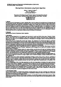
To avoid to write continuity conditions on the common vertices of the triangles of the mesh, one can find that in the n-th triangle of the points s,q,r (see Figure 1)

p

min ∫ ∇(∑ f n ) dv n

we find the equivalent minimization problem

min ∫ φ (un ) dv p

(9)

where φ (un ) is the function that we find after

replacing f n = an x + bn y + cn in ∇(∑ f n ) n

and an , bn , cn are evaluated using (8.1), (8.2), (8.3) for each triangle of the mesh.

Fig.1 A triangle in a 2-D mesh

u p = an xs + bn ys + cn

(7.1)

uq = an xq + bn yq + cn

(7.2)

ur = an xr + bn yr + cn

(7.3)

Equation (9) can be solved now by a variety of techniques. The author uses Genetic Algorithms with Nelder-Meade for Non-linear Problems as in [2], [3], [4], [5], [6], [7], [8]. The same optimization scheme: Genetic Algorithms with Nelder-Meade will be also applied for (9).

There three equations can be solved with respect to an , bn , cn and give

ISSN: 1109-2769

109

Issue 3, Volume 8, March 2009

WSEAS TRANSACTIONS on MATHEMATICS

Nikos E. Mastorakis

position in the sorted scores. The rank of the fittest individual is 1, the next fittest is 2 and so on. Rank fitness scaling removes the effect of the spread of the raw scores. Proportional Scaling Option: The Proportional Scaling makes the expectation proportional to the raw fitness score. This strategy has weaknesses when raw scores are not in a "good" range. Top Scaling Option: The Top Scaling scales the individuals with the highest fitness values equally.

Before proceeding in the solution of the problem, some background on GA (Genetic Algorithms) and Nelder-Mead is necessary. In [4], the author has also proposed a hybrid method that includes a) Genetic Algorithm for finding rather the neiborhood of the global minimum than the global minimu itself and b) Nelder-Mead algorithm to find the exact point of the global minimum itself. So, with this Hybrid method of Genetic Algorithm + Nelder-Mead we combine the advantages of both methods, that are a) the convergence to the global minimum (genetic algorithm) plus b) the high accuracy of the Nelder-Mead method.

Shift linear Scaling Option: The shift linear scaling option scales the raw scores so that the expectation of the fittest individual is equal to a constant, which you can specify as Maximum survival rate, multiplied by the average score. We can have also option in our Reproduction in order to determine how the genetic algorithm creates children at each new generation. For example, Elite Counter specifies the number of individuals that are guaranteed to survive to the next generation. Crossover combines two individuals, or parents, to form a new individual, or child, for the next generation. Crossover fraction specifies the fraction of the next generation, other than elite individuals, that are produced by crossover. Scattered Crossover: Scattered Crossover creates a random binary vector. It then selects the genes where the vector is a 1 from the first parent, and the genes where the vector is a 0 from the second parent, and combines the genes to form the child. Mutation: Mutation makes small random changes in the individuals in the population, which provide genetic diversity and enable the GA to search a broader space. Gaussian Mutation: We call that the Mutation is Gaussian if the Mutation adds a random number to each vector entry of an individual. This random number is taken from a Gaussian distribution centered on zero. The variance of this distribution can be controlled with two parameters. The Scale parameter determines the variance at the first generation. The Shrink parameter controls how variance shrinks as

If we use only a Genetic Algorithm then we have the problem of low accuracy. If we use only Nelder-Mead, then we have the problem of the possible convergence to a local (not to the global) minimum. These disadvantages are removed in the case of our Hybrid method that combines Genetic Algorithm with Nelder-Mead method. We recall the following definitions from the Genetic Algorithms literature:

Fitness function is the objective function we want to minimize. Population size specifies how many individuals there are in each generation. We can use various Fitness Scaling Options (rank, proportional, top, shift linear, etc), as well as various Selection Options (like Stochastic uniform, Remainder, Uniform, Roulette, Tournament). Fitness Scaling Options: We can use scaling functions. A Scaling function specifies the function that performs the scaling. A scaling function converts raw fitness scores returned by the fitness function to values in a range that is suitable for the selection function. We have the following options: Rank Scaling Option: scales the raw scores based on the rank of each individual, rather than its score. The rank of an individual is its

ISSN: 1109-2769

110

Issue 3, Volume 8, March 2009

WSEAS TRANSACTIONS on MATHEMATICS

Nikos E. Mastorakis

Step 1. Order. Order the n+1 vertices to satisfy f(x1) ≤ f(x2) ≤ … ≤ f(xn+1), using the tie-breaking rules given below. Step 2. Reflect. Compute the reflection point xr from xr = x + ρ ( x − x n +1 ) = (1 + ρ ) x − ρx n+1 ,

generations go by. If the Shrink parameter is 0, the variance is constant. If the Shrink parameter is 1, the variance shrinks to 0 linearly as the last generation is reached. Migration is the movement of individuals between subpopulations (the best individuals from one subpopulation replace the worst individuals in another subpopulation). We can control how migration occurs by the following three parameters. Direction of Migration: Migration can take place in one direction or two. In the so-called “Forward migration” the nth subpopulation migrates into the (n+1)'th subpopulation. while in the so-called “Both directions Migration”, the nth subpopulation migrates into both the (n-1)th

n

where x = ∑ xi / n is the centroid of the n best i =1

points (all vertices except for xn+1). Evaluate fr=f(xr). If f1 ≤ fr < fn , accept the reflected point xr and terminate the iteration. Step 3. Expand. If fr < f1 , calculate the expansion point xe, x e = x + χ ( x r − x ) = x + ρχ ( x − x n +1 ) = (1 + ρχ ) x − ρχx n +1

and the (n+1)th subpopulation. Migration wraps at the ends of the subpopulations. That is, the last subpopulation migrates into the first, and the first may migrate into the last. To prevent wrapping, specify a subpopulation of size zero. Fraction of Migration is the number of the individuals that we move between the subpopulations. So, Fraction of Migration is the fraction of the smaller of the two subpopulations that moves. If individuals migrate from a subpopulation of 50 individuals into a population of 100 individuals and Fraction is 0.1, 5 individuals (0.1 * 50) migrate. Individuals that migrate from

and evaluate fe=f(xe). If fe < fr, accept xe and terminate the iteration; otherwise (if fe ≥ fr), accept xr and terminate the iteration. Step 4. Contract. If fr ≥ fn, perform a contraction between x and the better of xn+1 and xr. Outside. If fn ≤ fr < fn+1 (i.e. xr is strictly better than xn+1), perform an outside contraction: calculate x c = x + γ ( x r − x ) = x + γρ ( x − x n +1 ) = (1 + ργ ) x − ργx n +1

one subpopulation to another are copied. They are not removed from the source subpopulation. Interval of Migration counts how many generations pass between migrations.

and evaluate fc = f(xc). If fc ≤ fr, accept xc and terminate the iteration; otherwise, go to step 5 (perform a shrink).

The Nelder-Mead simplex algorithm appeared in 1965 and is now one of the most widely used methods for nonlinear unconstrained optimization [33]÷[35]. The Nelder-Mead method attempts to minimize a scalar-valued nonlinear function of n real variables using only function values, without any derivative information (explicit or implicit).

b. Inside. If fr ≥ fn+1, perform an inside contraction: calculate x cc = x − γ ( x − x n +1 ) = (1 − γ ) x + γx n +1 , and evaluate

fcc = f(xcc). If fcc < fn+1, accept xcc and terminate the iteration; otherwise, go to step 5 (perform a shrink).

The Nelder-Mead method thus falls in the general class of direct search methods. The method is described as follows: Let f(x) be the function for minimization. x is a vector in n real variables. We select n+1 initial points for x and we follow the steps:

ISSN: 1109-2769

Step 5. Perform a shrink step. Evaluate f at the n points vi = x1 + σ (xi – x1), i = 2, … , n+1. The (unordered) vertices of the simplex at the next iteration consist of x1, v2, … , vn+1.

111

Issue 3, Volume 8, March 2009

WSEAS TRANSACTIONS on MATHEMATICS

Nikos E. Mastorakis

After this preparation, we are ready to solve the

min ∫ φ (un ) dv p

of (9) as minimization

problem.

The minimization is achieved by using Genetic Algorithms (GA) and the method of NelderMead exactly as we described previously. We can use the MATLB software package (MATLAB, Version 7.0.0, by Math Works). In the next numerical example (Section 3) our GA has the following Parameters Population type: Double Vector Population size: 30 Fig.2

Creation function: Uniform Fitness scaling: Rank

u = 0 in x = ±2, −2 ≤ y ≤ 2 y = ±2, −2 ≤ x ≤ 2

with

Selection function: roulette Reproduction: 6 – Crossover fraction 0.8

the

external

boundary:

and u = 1 in the internal boundary

Mutation: Gaussian – Scale 1.0, Shrink 1.0

x = ±1, −1 ≤ y ≤ 1 y = ±1, −1 ≤ x ≤ 1

Crossover: Scattered Migration: Both – fraction 0.2, interval: 20 Stopping criteria: 50 generations

3 Numerical Example Consider now the following problem (Fig.2)

(

div ∇u

p −2

)

∇u = 0

(4)

in the domain u ∈ [0, 2] × [0, 2] − [0,1] × [0,1]

Fig.3

Due to symmetry, we can split the domain in 8 same trapezoids (trapezia). It is sufficient to

ISSN: 1109-2769

112

Issue 3, Volume 8, March 2009

WSEAS TRANSACTIONS on MATHEMATICS

(

solve the problem div ∇u

p −2

Nikos E. Mastorakis

)

∇u = 0 in one of

them with the boundary conditions u = 0 in the external boundary and u = 1 in the internal boundary.

uq = an xq + bn yq + cn

(7.2)

ur = an xr + bn yr + cn

(7.3)

in every one of the 6 triangles, we solve as in (8.1), (8.2), (8.3) and finally we introduce to p J (u ) = ∫ ∇u dv (5) We have, considering also that u1 = u6 = 1 and

Taking one of these trapezoids and splitting it into 6 triangles like in Fig.3, we have in some enlargement the following Figure: Fig.4

u2 = u3 = u4 = 0 So, after some algebraic manipulation we find that we have to minimize the quantity I where p

I = 2u5 + 12 + (1 − 2u5 ) 2

p

+ 12 + (1 − 2u7 ) 2

p

+ (2 − 2u7 ) + 12 + (1 − 2u7 ) 2

p

+ (2u7 )

p

p

with respect to u5 , u7 Now, in order to find the global minimum of I we use GA (Population type: Double Vector Population size: 30 / Creation function: Uniform /Fitness scaling: Rank / Selection function: roulette / Reproduction: 6 – Crossover fraction 0.8 / / Mutation: Gaussian – Scale 1.0, Shrink 1.0 / / Crossover: Scattered / Migration: Both – fraction 0.2, interval: 20 /Stopping criteria: 50 generations) and continue with Nelder-Mead

Fig.4

We consider as u1 , u2 , u3 , u4 , u5 , u6 , u7 the value of the u at the points (0, 0), (2, 0), (2, 2), (2, 4), (1,3), (0, 2), (1,1) i.e.

So we find the following results for different values of p.

u1 = u (0, 0), u2 = u (2, 0),

p

u3 = u (2, 2),

2 3 4 5 6 7 8 10 20 50 200

u4 = u (2, 4), u5 = u (1,3), u6 = u (0, 2), u7 = u (1,1) Then by considering u p = an xs + bn ys + cn

ISSN: 1109-2769

(7.1)

113

u5 0.2500 0.3145 0.3471 0.3678 0.3824 0.3935 0.4024 0.4155 0.4468 0.4721 0.4903

u7 0.5000 0.5000 0.5000 0.5000 0.5000 0.5000 0.5000 0.5000 0.5000 0.5000 0.5000

I 5.5000 5.4623 5.4280 5.3994 5.3754 5.3550 5.3373 5.3082 5.2246 5.1375 5.0582

Issue 3, Volume 8, March 2009

+

WSEAS TRANSACTIONS on MATHEMATICS

Nikos E. Mastorakis

4 Solution of the equations (2), (3) and (4) We remind the problems: p−2 ∂ρ (1) = cα λ div ∇ρ n ∇ρ n , θ ∂t If we scale out the constants in (1), we derive ∂u = Δ p un (2) ∂t where a particular case of (2) is the nonNewtonian filtration equation ∂u = Δ pu (3) ∂t and ∂u p−2 (4) = div⎛⎜ ∇u ∇u ⎞⎟ + λu q , ⎝ ⎠ ∂t

)

(

( )

Consider that u can be written as u = ∑ λn (t ) f n or u = ∑ f n (t ) n

Fig.5

We express an (t ), bn (t ), cn (t ), d n (t ), en (t ), hn (t ) with respect not only u in vertices, but also in a node along the midside of each edge. See Fig.5. Finally using the so-called collocation method or least square method or the method of moments ([35]÷[40]) we can obtain a system of non-linear Ordinary Differential Equations that can be solved in a variety of methods (Runge – Kutta etc…).

where λn

n

have been incorporated to f n (t ) In this “dynamic” case, in a triangular mesh of 2 we can have f n = an (t ) x + bn (t ) y + cn (t ) for the n-th triangle. us = an (t ) xs + bn (t ) ys + cn (t ) uq = an (t ) xq + bn (t ) yq + cn (t )

(7.1) (7.2)

ur = an (t ) xr + bn (t ) yr + cn (t )

(7.3)

Of course, we can use higher polynomials like quadratic or cubic. For quadratic: us = an (t ) xs + bn (t ) ys + cn (t ) + d n (t ) xs2

5

Conclusion

In this paper, we have examined the boundary value problem

(

div ∇u

p −2

)

∇u = 0 where u

is a known function on the boundary of our domain using Variational Principle (Finite elements). The Problem is reduced to an Optimization problem that can be solved by Genetic Algorithms plus Nelder-Mead search. An early paper of the author with the title “Solving Differential Equations via Genetic

degree

Algorithms” was presented in [1] while the author use the same method to solve various problems in

[2]÷[9].

+ en (t )d + hn (t ) xs ys 2 s

ur = an (t ) xr + bn (t ) yr + cn (t ) + d n (t ) xr2

With the Hybrid method of Genetic Algorithm + Nelder-Mead we have combined the advantages of both methods, that are a) the convergence to the global minimum (genetic algorithm) plus b) the high accuracy of the Nelder-Mead method.

+en (t )d r2 + hn (t ) xr yr

Also, we have discussed briefly the solution of

uq = an (t ) xq + bn (t ) yq + cn (t ) + d n (t ) xq2 +en (t )d q2 + hn (t ) xq yq

( )

∂u = Δ p un ∂t

ISSN: 1109-2769

114

Issue 3, Volume 8, March 2009

WSEAS TRANSACTIONS on MATHEMATICS

Nikos E. Mastorakis

∂u = Δ pu ∂t and ∂u p−2 = div⎛⎜ ∇u ∇u ⎞⎟ + λu q , ⎝ ⎠ ∂t using the so-called collocation method or least square method or the method of moments.

AND SCIENTIFIC COMPUTATION (ISTASC'06), Elounda, Agios Nikolaos, Crete Island, Greece, August 21-23, 2006. 8. Nikos E. Mastorakis, “Unstable Ordinary Differential Equations: Solution via Genetic Algorithms and the method of Nelder-Mead”, The 6th WSEAS International Conference on SYSTEMS THEORY AND SCIENTIFIC COMPUTATION, Elounda, Agios Nikolaos, Crete Island, Greece, August 18-20, 2006. 9. Nikos E. Mastorakis, “Unstable Ordinary Differential Equations: Solution via Genetic Algorithms and the Method of Nelder-Mead”, WSEAS TRANSACTIONS on MATHEMATICS, Issue 12, Volume 5, December 2006, pp. 12761281. 10. Nikos E. Mastorakis, “An Extended CrankNicholson Method and its Applications in the Solution of Partial Differential Equations: 1-D and 3-D Conduction Equations”, WSEAS TRANSACTIONS on MATHEMATICS, Issue 1, Volume 6, January 2007, pp. 215-224. 11. Saeed-Reza Sabbagh-Yazdi, Behzad Saeedifard, Nikos E. Mastorakis, “Accurate and Efficient Numerical Solution for Trans-Critical Steady Flow in a Channel with Variable Geometry”, WSEAS TRANSACTIONS on APPLIED and THEORETICAL MECHANICS, Issue 1, Volume 2, January 2007, pp. 1-10. 12. Saeed-Reza Sabbagh-Yazdi, Mohammad Zounemat-Kermani, Nikos E. Mastorakis, “Velocity Profile over Spillway by Finite Volume Solution of Slopping Depth Averaged Flow”, WSEAS TRANSACTIONS on APPLIED and THEORETICAL MECHANICS, Issue 3, Volume 2, March 2007, pp. 85. 13. Iurie Caraus and Nikos E. Mastorakis, “Convergence of the Collocation Methods for Singular Integrodifferential Equations in Lebesgue Spaces”, WSEAS TRANSACTIONS on MATHEMATICS, Issue 11, Volume 6, November 2007, pp. 859-864. 14. Iurie Caraus, Nikos E. Mastorakis, “The Stability of Collocation Methods for Approximate Solution of Singular Integro- Differential Equations”, WSEAS TRANSACTIONS on MATHEMATICS, Issue 4, Volume 7, April 2008, pp. 121-129. 15. Xu Gen Qi, Nikos E. Mastorakis, “Spectral distribution of a star-shaped coupled network”, WSEAS TRANSACTIONS on APPLIED and THEORETICAL MECHANICS , Issue 4, Volume 3, April 2008. 16. Iurie Caraus, Nikos E. Mastorakis, “Direct Methods for Numerical Solution of Singular

References: 1. Nikos E. Mastorakis, “Solving Differential Equations via Genetic Algorithms”, Proceedings of the Circuits, Systems and Computers ’96, (CSC’96), Piraeus, Greece, July 15-17, 1996, 3rd Volume: Appendix, pp.733-737 2. Nikos E. Mastorakis, “On the solution of illconditioned systems of Linear and Non-Linear Equations via Genetic Algorithms (GAs) and Nelder-Mead Simplex search”, 6th WSEAS International Conference on EVOLUTIONARY COMPUTING (EC 2005), Lisbon, Portugal, June 16-18, 2005. 3. Nikos E. Mastorakis, “Genetic Algorithms and Nelder-Mead Method for the Solution of Boundary Value Problems with the Collocation Method”, WSEAS Transactions on Information Science and Applications, Issue 11, Volume 2, 2005, pp. 2016-2020. 4. Nikos E. Mastorakis, “On the Solution of Ill-Conditioned Systems of Linear and Non-Linear Equations via Genetic Algorithms (GAs) and Nelder-Mead Simplex Search”, WSEAS Transactions on Information Science and Applications, Issue 5, Volume 2, 2005, pp. 460-466. 5. Nikos Mastorakis, “Genetic Algorithms and Nelder-Mead Method for the Solution of Boundary Value Problems with the Collocation Method”, 5th WSEAS International Conference on SIMULATION, MODELING AND OPTIMIZATION (SMO '05), Corfu Island, Greece, August 17-19, 2005. 6. Nikos E. Mastorakis, “Solving Non-linear Equations via Genetic Algorithm”, WSEAS Transactions on Information Science and Applications, Issue 5, Volume 2, 2005, pp. 455459. 7. Nikos E. Mastorakis, “The Singular Value Decomposition (SVD) in Tensors (Multidimensional Arrays) as an Optimization Problem. Solution via Genetic Algorithms and method of Nelder-Mead”, 6th WSEAS Int. Conf. on SYSTEMS THEORY

ISSN: 1109-2769

115

Issue 3, Volume 8, March 2009

WSEAS TRANSACTIONS on MATHEMATICS

Nikos E. Mastorakis

Integro-Differentiale Quations in Classical (case γ ≠ 0)”, 10th WSEAS International Conference on MATHEMATICAL and COMPUTATIONAL METHODS in SCIENCE and ENGINEERING (MACMESE'08), Bucharest, Romania, November 7-9, 2008. 17. Gabriella Bognar, Numerical and

29. W. L. Wood, Introduction to Numerical

Methods for Water Resources, Oxford University Press, 1993 30. Daniel R. Lynch, Numerical Partial Differential Equations for Environmental Scientists and Engineers: A First Practical Course, Springer, 2005

Numerical and Analytic Investigation of Some Nonlinear Problems in Fluid Mechanics, COMPUTER and SIMULATION in MODERN SCIENCE, Vol.II, WSEAS Press, pp.172-179, 2008 18. Astrita G., Marrucci G., Principles of NonNewtonian Fluid Mechanics, McGraw-Hill, New York, NY, USA, 1974. 19. Volquer R.E., Nonlinear flow in porous media by finite elements, ASCE Proc., J. Hydraulics Division Proc. Am. Soc. Civil Eng., 95 (1969), 2093-2114 20. Ahmed N., Sunada D.K., Nonlinear flow in porous media, J. Hydraulics Division Proc. Am. Soc. Civil Eng., 95 (1969), 1847-1857. 21. Peebles P.J.E., Star distribution near a collapsed object, Astrophysical Journal, Vol. 178, (1972),. 371-376. 22. Carelman T., Probl`emes math´ematiques dans la th´eorie cin´etique de gas, AlmquistWiksells, Uppsala, 1957. 23. Bartnik R., McKinnon J., Particle-like solutions of the Einstein-Yang-Mills equations. Phys. Rev. Lett. 61 (1988), 141-144 24. Otani M., A remark on certain nonlinear elliptic equations. Proc. Fac. Sci. Tokai Univ. 19 (1984), 23--28. 25. Pelissier, M.-C., Reynaud, L., Étude d'un modèle mathématique d'ecoulement de glacier, C. R. Acad. Sci., Paris, Sér. A 279 (1974), 531534. (French) 26. Schoenauer M., A monodimensional model for fracturing, In A. Fasano and M. Primicerio (editors): Free Boundary Problems, Theory Applications, Pitman Research Notes in Mathematics 79, Vol. II., London, 701-711 (1983). 27 John C. Strikwerda, Finite Difference Schemes and Partial Differential Equations, SIAM, 2004 28. Hans Petter Langtangen Computational Partial Differential Equations: Numerical Methods and Diffpack Programming, Springer, 2003

ISSN: 1109-2769

31. Nikos E. Mastorakis, “Numerical Schemes for Non-linear Problems in Fluid Mechanics”, Proceedings of the 4th IASME/WSEAS International Conference on CONTINUUM MECHANICS, Cambridge, UK, February 24-26, 2009, pp.56-61 32. Evans, Lawrence C. , A New Proof of Local C1,α Regularity for Solutions of Certain Degenerate Elliptic P.D.E.", Journal of Differential Equations 45: 356-373, 1982 32. Lewis, John L. (1977). Capacitary functions in convex rings, Archive for Rational Mechanics and Analysis 66: 201–224, 1977 33. Lagarias, J.C., J. A. Reeds, M. H. Wright, and P. E. Wright, "Convergence Properties of the Nelder-Mead Simplex Method in Low Dimensions," SIAM Journal of Optimization, Vol. 9 Number 1, pp. 112-147, 1998 34. J. A. Nelder and R. Mead, “A simplex method for function minimization”, Computer Journal, 7 , 308-313, 1965 35. F. H. Walters, L. R. Parker, S. L. Morgan, and S. N. Deming, Sequential Simplex Optimization, CRC Press, Boca Raton, FL, 1991 36.A. Ern, J.L. Guermond, Theory and practice of finite elements, Springer, 2004, ISBN 0-3872-05748 37. S. Brenner, R. L. Scott, The Mathematical Theory of Finite Element Methods, 2nd edition, Springer, 2005, ISBN 0-3879-5451-1 38. P. G. Ciarlet, The Finite Element Method for Elliptic Problems, North-Holland, 1978, ISBN 04448-5028-7 39 Y. Saad, Iterative Methods for Sparse Linear Systems, 2nd edition, SIAM, 2003, ISBN 0-89871534-2 40. J.J.Conor and C.A.Brebbia, Finite Element Techniques for Fluid Flow, Butterworth, London, 1976

116

Issue 3, Volume 8, March 2009