GENETIC OPERATORS AND CONSTRAINT HANDLING FOR PIPE NETWORK OPTIMIZATION Dragan A. Savic1 and Godfrey A. Walters School of Engineering Exeter, UK
ABSTRACT Evolution Programs (EPs), including Genetic Algorithms and Evolution Strategies, are well-suited for pipe network optimization problems due to the large number of candidate solutions to be examined, non-linearity of the problem and discrete decision space. However, pipe network problems are highly constrained and random initialization and standard genetic operators often cause infeasibility of generated solutions. The paper describes coding and genetic operators adapted to preserve feasibility of pipe network solutions generated in an EP run. Examples of ‘hard’ and ‘soft’ constraints found in pipe network optimization problems are used to illustrate the coding and genetic operators developed. The ‘hard’ constraints must be satisfied for each candidate solution and the ‘soft’ constraints may be violated but with a penalty associated with the violation. Procedures devised to include different type of constraints into an EP structure are also summarized. Examples of EPs developed include: (1) optimal pipe sizing for water distribution networks (2) layout design of branched hydraulic networks; and (3) pressure regulation in water distribution networks. The first example involves a classical operational-research type constraint of the form f(x) ≥ b. The second example involves a topological (connectivity) constraint which ensures that all nodes are connected (supplied). The last example combines the two constraints in a single problem. The examples provided clearly demonstrate the ability of the EPs developed to find solutions to problems difficult to solve using classical operational research methods. INTRODUCTION The production and distribution of gas is a very important factor in Britain’s economy. Similarly, the water industry provides one of the most significant services to the public. Common components of gas and water systems are pipe networks whose design and management costs are often immense. Consequently various methodologies for the economic and efficient design of pipe networks have been developed over the years as reported by Walters and Savic (1). Their review shows that optimization of water networks has been receiving a considerable amount of interest for more than thirty years. However, optimal design of pipe networks belongs to the class of large NP-hard problems which are difficult to solve using classical operational research techniques. After reported successful applications in many problem domains, pipe network optimization has started to benefit from the use of computer algorithms mimicking certain principles of nature. The particularly useful principles were observed in annealing processes, central nervous systems and biological evolution, which in turn have lead to the following optimization methods: Simulated Annealing (SA), Artificial Neural Networks (ANNs) and Evolution Programs (EPs). Evolution Programs, of which Genetic 1
[email protected] 1
Algorithms (GA) and Evolution Strategy (ES) are best known, are general artificialevolution search methods based on natural selection and the mechanisms of population genetics. Evolution Programs are well-suited for pipe network optimization problems due to the large number of candidate solutions to be examined, non-linearity of the problem and discrete decision space. The choice of EP structure and parameters involves the following decisions: (1) The most appropriate form of coding or data structure to define the design variables. (2) The means for generating an initial population of feasible solutions. (3) The population size to adopt. (4) The form of fitness function to be used. (5) The way in which ‘parents’ are chosen and ‘children’ generated, including decisions on preferential selection, crossover and mutation. (6) The way in which the members of a population are replaced. (7) Criteria for termination of the process. This paper puts emphasis on coding and genetic operators specifically developed to preserve feasibility of pipe network solutions generated in an EP run. It also describes procedures devised to include different type of constraints into an EP structure. These two topics are presented using examples of EPs developed for: (1) optimal pipe sizing for water distribution networks (2) layout design of branched hydraulic networks; and (3) pressure regulation in water distribution networks. The first example involves a classical operational-research type constraint of the form f(x) ≥ b. The second example involves a topological (connectivity) constraint which ensures that all nodes are connected (supplied). The last example combines the two constraints in a single problem. OPTIMAL PIPE SIZING Problem Statement Design of water distribution networks is often viewed as a least-cost optimisation problem with pipe diameters being decision variables. Pipe layout, connectivity and imposed minimum head constraints at pipe junctions (nodes) are considered known. There are obviously other possible objectives, like reliability, redundancy and/or water quality, that can be included in the optimisation process. However, problems with quantifying these objectives for use within optimisation design models kept researchers concentrating on a single, least-cost objective. Even that, restricted formulation of the optimal network design represents a difficult problem to solve. The following mathematical statement of the optimal design problem is presented for a general water supply network. The objective function is usually a cost function of pipe diameters and lengths N
f ( D1 ,..., Dn ) = ∑ c( Di , Li )
(1)
i=1
where c(Di, Li) is the cost of the pipe i with the diameter Di and the length Li, and N is the total number of pipes in the system. The above function is to be minimised under the following constraints.
2
For each junction node (other than the source) a continuity constraint should be satisfied
∑Q −∑Q in
out
= Qe
(2)
where Qin is the flow into the junction, Qout is the flow out of the junction and Qe represents the external inflow or demand at the junction node. Under this convention demands Qe which extract flow from the junction are positive. For each of the basic loops in the network the energy conservation constraint can be written as:
∑ h −∑ E f
p
=0
(3)
where Ep is the energy put into the liquid by a pump. If more than one source nodes are available then an additional energy conservation constraint is written for paths between any two of the nodes. The Hazen-Williams formula is used to express the energy loss term hf
hf =
L a b Q C D
(4)
a
where the coefficient a equals 1/0.54, the coefficient b equals 2.63/0.54, L is the length of the pipe, C is the Hazen-Williams coefficient, D is the diameter of the pipe and Q is the flow. The minimum head constraint for each node in the network is given in the form
H j ≥ H jmin ; j = 1,..., M
(5)
where Hj is the head at node j, Hjmin is the minimum required head at the same node, and M is the total number of nodes in the system. The optimisation problem formulated in this manner is non-linear due to energy conservation equations. In addition, pipes for water supply are manufactured in a set of discrete-sized diameters thus introducing additional difficulties to the problem of searching for the optimal design. Constraint Handling The EP adopted for this problem was a Gray-coded GA coupled with an efficient hydraulic solver used to calculate heads and flows in a network. The solver ensures that the constraints of Eqs.(2) and (3) are satisfied for each generated solution. The minimum pressure constraint of Eq. (5) is not necessarily satisfied and it discriminates between feasible and infeasible solutions. Rather than ignoring the infeasible solutions, and concentrating only on feasible ones, infeasible solutions are allowed to join the population and help guide the search, but for a certain price. A penalty term incorporated in the fitness function is activated for a pressureinfeasible solution thus reducing its strength relative to the other strings in the population
[ (
)]
N f ( D1 ,..., Dn ) = ∑ c( Di ) × Li + p ⋅ max max H j min − H j ,0 j i =1
(6)
3
where p is the penalty multiplier and the term in brackets is the maximum violation of the pressure constraint. The penalty multiplier is chosen to normalise nominal values of the penalties to the same scale as the basic cost of the network.
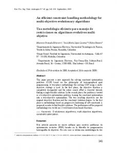
Figure 1. The Hanoi network The multiplier is a function of the generation number which allows a gradual increase of the penalty term
p = pc ⋅ f ( n gen )
(7)
where pc is the constant penalty multiplier, ngen is the generation number and f is a monotonically increasing function. At the end of a GA run, the multiplier p should take a value which will not allow the best infeasible solution to be better than any feasible solution in the population. Savic and Walters (2) used the above GA to analyze several pipe sizing problems 9 from the literature. The problems analyzed vary in size from 1.5×10 possible designs (a network consisting of 7 nodes, 8 pipes and two loops with 14 discrete diameters considered) to 2.9×1026 possible designs (the Hanoi network in Figure 1 consisting of 32 nodes, 34 pipes and 3 loops with 6 discrete diameters considered). They found that GA solutions compared favourably in terms of cost and minimum head requirements to those obtained by several other techniques.
LAYOUT DESIGN OF BRANCHED HYDRAULIC NETWORKS Problem Statement The network layout describing the structure of a pipe system represents one of the main network features. The earliest optimization models for water distribution networks were developed for branched network layouts. In these tree-like systems,
4
a given demand pattern defines the flows in the pipes explicitly and uniquely. In a looped network there are infinite number of distributions of flow which can meet the demand pattern. One possible aim of optimising the layout of a branched network is to select the minimum cost set of arcs that is necessary to supply all given demands. Walters and Lohbeck (3) analysed the layout problem of branched networks for water, gas and sewer systems. The optimisation problem was defined as a search for the best tree layout from a directed base graph of possible pipeline connections (Figure 2). The main assumption of the method employed was that flow directions in the base graph are specified in advance. The simplification of using a directed base graph greatly reduces the number of candidate solutions, i.e., tree-like networks. The authors have shown that for a 25-node grid network (whose nodes are located in a rectangular pattern with each node served by at most two upstream arcs) the assumption of flow directions reduces the search space from approximately 3.3 × 10¹³ possible layouts to about 3.4 × 10⁷ possibilities. Even for this small example the solution space still remains large with a great number of local minima.
Figure 2. An example of a directed base graph and a possible branched network In order to determine the cost of a network layout a simplified cost function is used. Assuming a constant pressure gradient in a pipe system, a concave function in terms of length and flow is a reasonable approximation to express the cost of the system N
Cost = ∑ Li ⋅ Qi
(8)
i=1
Constraint Handling - Directed Graph As the target was to create a least-cost layout that connects all given nodes an obvious constraint to the problem was to generate only feasible candidate solutions,
5
i.e., whose base graph is connected. In order to satisfy this constraint under all circumstances and to take advantage of binary coding, the following problem formulation was developed. Since a conventional binary representation fits well when not more than two possible pipes converge on a node the formulation was developed to accommodate that constraint. The binary string used can be viewed as an array of one-bit elements, one for each node with two upstream pipes. For example, string S = [∗∗∗∗∗], where ∗ can be 0 or 1, represents a network whose 5 nodes have two alternative supply links each. In a tree each node has just one upstream pipe. Thus, each element of the string specifies which of the two upstream pipes will remain in the solution. It should be noted that nodes with just one upstream link are not included in the string since there is no alternative supply route. However, most of the real networks are irregular, i.e., they contain nodes with more than two upstream links. Therefore, additional intervention is needed if the simple binary mapping of one decision per bit is to be preserved. The solution was found in the form of dummy nodes. These nodes with zero demand are introduced into the base graph so that at most two links converge on each node. In addition, these nodes are located exactly in the same position as the original ones. No domain-specific genetic operators were employed since the formulated problem fitted exactly the standard GA paradigm. There are however concerns about the efficiency of the standard GA for base graphs with more than two alternative links supplying each node. In addition, the problem of uneven representation of integer choices using a binary coding and dummy nodes can also reduce the efficiency of the standard GA. Therefore, an alternative to the binary representation of the network layout was developed using integer mapping. An integer string is used to represent the possible incoming pipe links. The integer coding ensures equality of choice at a node, i.e., all links are equally likely to be included in a randomly generated network. When tested on the same examples as the standard GA the integer-coded GA was found to achieve on average better solutions. This was particularly true for highly connected networks while for sparsely connected networks improvements ranged from moderate to negligible. Both GA formulations compared favourably to the direct Dynamic Programming (DP) approach which is guaranteed to produce the global minimum cost solution. However, because of the well-known “curse of dimensionally” the possible network size that can be tackled with DP for layout optimisation is very limited. Undirected base-graph networks are not only larger problems to solve but also pose more difficulties than directed networks. These problems are highly constrained since the connectivity of the network has to be preserved. Walters and Smith (4) also used an integer-coded EP for the selection of a branched network from a nondirected base graph. The program developed ensures the generation of feasible solutions. This is achieved through innovative coding, recombination and mutation operators. Genetic Operators and Constraint Handling - Undirected Graphs Instead of using a single set of integers as in case of directed networks, the basegraph of an undirected network is represented using two sets of integers A and A. The first set, A, defines all arcs in the graph with the original (arbitrarily assigned) flow directions. The second set, A, defines all arcs in the graph that have directions opposite to those originally defined. An arc that belongs to neither set does not exist in the graph, and one that belongs to both is an undirected arc. A tree-growing 6
algorithm was devised to produce a spanning tree on a random basis from a base graph which can contain a mixture of directed and undirected arcs. The classical crossover operator was not applicable for this case since it would cause infeasibility of the offspring. Instead, the ‘genetic pool’ is formed by simple addition of the appropriate arc sets of the parents chosen from the population:
P = Ai + Aj, P = Ai + Aj.
(9)
The complete ‘genetic’ information about the design of an individual is contained in the two sets of arcs. This operation preserves the connectivity of the graph and allows the tree-growing algorithm to produce feasible offspring from the genetic pool. Mutation is performed by adding at random one or more directed arcs onto the graph. This means randomly adding extra elements to the pool of genetic information. By running the program a large number of times on different networks and with different population sizes and mutation rates, the best EP parameters were identified. It was found that a population of n = 16-20 and mutation rate averaging about one additional arc added to the genetic pool were the most effective. The program was successfully applied to a two-source example problem with 100 nodes and 232 arcs (3.65×1054 possible solutions). To reach the best identified solution each run required on average 32000 evaluations of network cost, 50 orders of magnitude fewer than for complete enumeration of the problem. When solutions obtained from the directed and undirected base graph problems were compared it was found that the new EP had identified less expensive designs. PRESSURE REGULATION IN WATER DISTRIBUTION NETWORKS Problem Statement As sections of the network may have to be isolated to repair leaks or for other purposes, isolating valves are frequently installed at specific intervals, the spacing being dependent on cost and operational considerations. Closing one or more of these valves without isolating any part of the network changes the configuration and hence the distribution of flows and pressures in the whole system. If nodal requirements (i.e. demand and minimum pressure head) stay unchanged, the problem can be posed as: find the optimal settings of all isolating valves (i.e., open or closed) to attain the best possible pressure distribution without compromising network performance (i.e., required flow is supplied to each node and minimum head requirement is satisfied). The objective function for this optimisation problem is given in the form N
min J = ∑ H i − H imin
CV ⊆V
(10)
i=1
where V is a set of all valves in the network, and CV is a set of closed valves. The minimum head constraint is the same as in Eq.(5).
Genetic Operators and Constraint Handling Savic and Walters (5) used a set of integer numbers to represent pipes which supply water to the network nodes. A single set (chromosome) completely defines 7
which arcs are closed (no-flow pipes) and which are not. Furthermore, the set A with pipes which are not closed is divided into two subsets, one consisting of the arcs that constitute a spanning tree, At, and the other which contains the remainder of the set (i.e., a co-tree), Act. This division of the set A is adopted to ensure creation of feasible (connected) network layouts from the network base graph and also to set up the equations for hydraulic analysis (node and loop equations). The creation of the ‘genetic’ pool is performed by simply adding two parent chromosomes. A random tree-growing algorithm is used to grow a tree through the available arcs and identify a tree set of a child. This step ensures feasibility (connectedness) of the child. It is also reasonable to assume that arcs which are common to both parents but not included in the tree should stay in the genetic material conveyed to the child. This is achieved by creating the co-tree set comprising these arcs. In addition, some of the arcs which were present in one or the other parent are added to the co-tree set with the probability p = 0.5. To allow for an operation similar to mutation in standard GA an arc is permitted to be added or taken out from the co-tree set (with low probability). To illustrate how difficult it is to generate a feasible solution without the above methodology an example with 47 pipes is used (Figure 3). The number of possible candidate solutions is 1.4×10¹⁴ (247). However, by evaluating a large number of solutions created by random valve closures it was found that, on average, only 1 in 10,000 generated solutions is connected. Although the above genetic operators take care of topological constraints there is still the minimum head constraint to be satisfied. Since solutions infeasible with regards to Eq.(5) may still be useful in the search they are not simply discarded. Instead, the constrained problem is transformed into an unconstrained problem by associating a penalty with constraint violation. The non-negative penalty function is given as
P = ∑ α ⋅ ( H imin − H i )
(11)
i∈ I v
where Iv is the set of nodes for which the minimum head constraint is violated and α is a positive penalty multiplier. The objective function takes a new compounded form
min J = P + ∑ ( H i − H imin )
CV ⊆V
(12)
i∈ I
where I is the set of nodes for which the minimum head constraint is satisfied. To assess the reduction in excess pressures, the pressure distribution for the example problem (Figure 3) is first obtained for the case where there are no closed valves in the network. The objective function value for this case of no pressure control is J = 1257.5 m. By repeatedly running the EP with the same parameters as in the first example, the lowest objective function value was found to be J = 473.7 m.
8
Figure 3. A network example for pressure regulation The best solution identifies closure of 9 valves. In contrast, an alternative, nearoptimal solution, having an objective function value of J = 476.2 m, identifies a very different set of 10 valves. If a smaller number of valves is more desirable, then a solution which requires only 5 valves to be closed can be used. The objective function value for this solution (J = 494.3 m) is only 4.3% greater than that for the best solution found. In addition, if solutions which are infeasible with respect to the minimum head requirement are analysed, those with relatively small minimum head violations may be considered acceptable in some circumstances. For example one such solution is to close valves [4, 7, 26, 37, 47]. This gives an objective function value of J = 371.0 m, an improvement of 21.7% over the best solution identified but with a minimum head violation of 2.0 m at node 31. It is also important to note that the EP was allowed 50,000 evaluations (number of generations × number of members in a population) per run which represents only 0.00036% of the expected number of feasible (connected) networks. CONCLUDING REMARKS Evolutionary computing is an area which promises to bridge the gap between researchers and practitioners dealing with pipe network optimization. The examples provided in this paper clearly demonstrate the ability of EPs to find solutions to problems difficult to solve using classical operational research methods. The power of Evolutionary methods has already captured the imagination of the research community and their conceptual simplicity will certainly appeal to practitioners. The paper gives examples of ‘hard’ and ‘soft’ constraints found in pipe network optimization problems. The former must be satisfied for each candidate solution and the latter may be violated but with the penalty associated with the constraint 9
violation. A standard GA was found not to be adequate for the three problems considered. The authors had to apply not only the non-binary coding but also to devise domain-specific genetic operators to include hard constraints into problem formulation. Soft constraints were dealt with using EPs with penalties which are functions of the distance from feasibility. Where possible starting with relaxed constraints and tightening them as the run progresses was also applied. ACKNOWLEDGEMENT This work was supported by the UK Engineering and Physical Sciences Research Council, grant GR/J09796. REFERENCES 1. Walters, G.A. and Savic, D.A., (1994), Optimal Design of Water Systems using Genetic Algorithms and Other Evolution Programs, Keynote paper in Hydraulic Engineering Software V Vol.1: Water Resources and Distribution, W.R. Blain and K.L. Ktsifarakis (eds.), Computational Mechanics Publications, pp.19-26. 2. Savic, D.A. and Walters, G.A., (1994), Sensitivity of Optimal Pipeline System Designs to Changes in Head-Loss Equation, Centre For Systems And Control Engineering, Report No. 94/21, School of Engineering, University of Exeter, Exeter, United Kingdom. 3. Walters, G.A. and Lohbeck, T.K., (1993), Optimal layout of tree networks using genetic algorithms, Engineering Optimization, 22, pp.27-48. 4. Walters, G.A. and Smith, D.K., (1995), Evolutionary design algorithm for optimal layout of tree networks, Engineering Optimization, (in press). 5. Savic, D.A. and Walters, G.A., (1995), An Evolution Program for Optimal Pressure Regulation in Water Distribution Networks, Engineering Optimization (in press).
10