Genetic Programming for Improved Data Mining -Application to the Biochemistry of Protein Interactions M.L. Raymer1,3
W.F. Punch1
E.D. Goodman2
1Computer Science Department, A714 Wells Hall, {raymermi,punch}@cps.msu.edu 2 Case Center for Computer Aided Engineering and Manufacturing, 112 Engineering
L.A. Kuhn3 Building,
[email protected] 3 Department of Biochemistry, 502 Biochemistry Building,
[email protected] Michigan State University, East Lansing MI, 48824
ABSTRACT We have previously shown how a genetic algorithm (GA) can be used to perform “data mining,” the discovery of particular/important data within large datasets, by finding optimal data classifications using known examples. However, these approaches, while successful, limited data relationships to those that were “fixed” before the GA run. We report here on an extension of our previous work, substituting a genetic program (GP) for a GA. The GP could optimize data classification, as did the GA, but could also determine the functional relationships among the features. This gave improved performance and new information on important relationships among features. We discuss the overall approach, and compare the effectiveness of the GA vs. GP on a biochemistry problem, the determination of the involvement of bound water molecules in protein interactions.
1. Introduction A rigorous definition of the term data mining is difficult, but it has come to mean a search through a large database for “nuggets” of information that can be used for some particular purpose. We have previously addressed data mining problems using a genetic algorithm(GA). We view the problem of data mining as a problem of feature extraction, which we optimize with a GA. Two results are generated: • a list of features which are important for distinguishing the particular data from the background of the large database, and a (typically much larger) list of features which are not important for distinguishing the data. • of those important features, a relative weighting indicative of their importance for distinguishing the data. The rest of this paper will review: feature extraction, our
approach to optimizing feature extraction using a GA, our improved approach using a genetic program (GP), and an example of the effectiveness of both the GA and the GP on an important biochemistry problem, using the chemistry of proteins to predict their binding to other molecules.
2. The Basis for the Approach 2.1
Feature Extraction
Our data mining approach is based on feature extraction as described in classical pattern recognition literature. Broadly speaking, there are two steps: identification of the features and their form to be used in the recognition, thus defining the feature space, and the formation of the classification or decision rules used to separate the pattern classes in the feature space. Definition of the feature space can be a difficult problem. Too few features (or non-representative features) may not provide enough information on which to base classification while too many features make the search process intractable. The rapid growth in the search space as additional features are added, which also increases the number of training samples required, is often referred to as the curse of dimensionality. Feature selection methods attempt to find the best subset of size d of features of the original N features. “Best” is typically defined as that subset of cardinality d which gives the best classification (fewest misclassifications). Since an enumerative search of all size d subsets is computationally infeasible (essentially N ), at least for any reasonably sized N, there d are a number of heuristic approaches that have been used, including sequential forward selection[Jain82], branch and bound[Narendra77] and GA’s[Siedlecki89, Kelly91, Punch93]. Feature extraction methods define a transformation to the feature space such that fewer features are required and the features used give better separation of the pattern classes. Thus feature extraction subsumes feature selection. Feature extraction is the approach we will focus on here. Formally (following the work of Devivjer and Kittler[Devivjer82]), we can define the set of features used in classification as a vector y. The goal of feature extraction is to
= Type X
define a new feature vector yˆ that meets the criterion for improved classification. We accomplish this transformation by defining a mapping function W() such that yˆ = W ( y ) .
= Type Y = Type
The result of applying W() is both to create yˆ such that yˆ ≤ y and to increase separation of pattern classes in the
Unknown
feature space as now defined by yˆ . Formally, we define W() by optimizing a criterion function J(), ideally the probability of correct classification. Selection of W(y) is defined as the optimal transformation among all possible transformations ˆ ( y ) such that: W
Feature A
ˆ ( y) } ) J { W ( y ) } = max(J { W While W() could consist of any transform, in the classification literature it typically is a linear mapping. 2.2
Using a GA for Feature Extraction
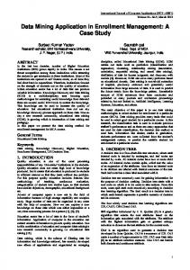
The essence of our earlier approach to feature extraction is twofold: • Modify the original feature space based on a vector of weights generated by a genetic algorithm. • Use a K-nearest-neighbor algorithm to evaluate the effectiveness of the weight vector in increasing separation between known pattern classes. A Knn is a simple rule for classification, and its general approach is shown in Figure 1. Each feature of the test set is a dimension in the classification search space. For simplicity’s sake, let us assume that there are only two features in the test we conduct, represented by the x and y axes in the figure. Known examples are then placed into this space as points based on their known feature values and labeled according to their known classification. An unknown can then be placed in the same space based on its feature values, and it can be classified based on its K nearest neighbors, where K is set to some integer value. Assume K=3; then in Figure 1, the unknown sample is labeled as type X based on the fact that 2 of its 3 nearest neighbors are of type X. Our hybrid GA-Knn approach (see [Punch93] for more details) was inspired by work first reported by Siedlecki and Sklansky [Siedlecki89] but modifies and extends their approach in several ways. Siedlecki and Sklansky’s goal was to find “the smallest or least costly subset of features for which the classifier’s performance does not deteriorate below a certain specified level”[Siedlecki89]. This was done by constructing a GA chromosome which consisted of a binary encoding whose length (in bits) equaled the number of features. If a bit equaled one, that feature was preserved in the feature space and used by the Knn to classify exemplars into pattern classes. Each such string was penalized based on its performance (more penalty for worse performance in classifying the exemplars) and its length (more penalty for more 1’s in the chromosome). Their approach was as good as many standard approaches, such as exhaustive search and branch and bound, and much better on large feature sets (20 features or more) where the standard approaches showed poor computational performance.
3 Nearest Neighbors
Feature B
Figure 1 An example Knn classification. The unknown is classified as type X based on the majority of its K (in this case three) nearest neighbors. The Siedlecki-Sklansky chromosome is an example of a 0/ 1 weighting of the importance of the features. That is, the feature space of the samples is uniformly modified by multiplying each exemplar’s feature vector y by the GA weight vector w (in this case 0 or 1) and this modified Knn rule is used to classify the known samples via Knn. Thus the SiedleckiSklansky approach is one of feature selection. We modified this approach to perform feature extraction by allowing the weights to be real values ranging over a broader scale, such as 0 to 10. Features are prenormalized to the range [1,10], giving the weights an interpretation of the relative importance of features to the classification task by scaling that feature’s axis. Our feature extraction searches for a relative weighting of features that gives optimal performance on classification of the known samples. Those weights that move towards 0 indicate that their corresponding features are not important for discrimination, and any weight that moves towards the maximum indicates that the classification is sensitive to small changes in that feature. Thus each feature’s dimension is elongated or shortened according to its importance in classification. Similar work was pursued by Kelly and Davis[Kelly91]. GA-Knn feature extraction is therefore a scaling of the feature space such that an optimal class separation can be achieved between the known classes. This weighting vector, once discovered, can then be used independently of the GA to classify unknown samples and can also be used to indicate which differences are important for class separation, providing focal points for further research in the application area. 2.3 Formal Definition of Feature Extraction for GA-Knn From the definitions shown in Section 2.1, we formally describe the problem by defining the functions W() and J().
Table
1:
Results of Training and Unbiased Testing of Waters Displacement using the GA-Knn Training Set
Water Status Conserved (Predicted/Observed)
Displaced (Predicted/Observed)
1700 waters (including 157 active site waters used for testing), k=3, (biased test)
35/42, (83%)
86/115, (75%)
121/157, (77.1%)
1700 waters (with same 157 active waters), k=3, (test 67 unknown active site waters)
11/16, (69%)
39/51, (76%)
50/67, (74.6%)
• The criterion function J() used is the performance of the Knn in properly classifying exemplars into pattern classes. The Knn is run on this new feature space and misclassifications noted. The w giving the fewest misclassifications is considered the “optimal” transformation. Using the GA-Knn to Predict Protein Interactions
We tested the GA-Knn system on both artificially generated test data and on real-world application data. The approach proved particularly effective on “noisy” data, that is data where class exemplars had some random variance. We have applied it in areas such as: classification of soil samples based on microbial populations [Punch93], classification of characteristics of microbes with certain abilities (such as pesticide degradation and organic chemical degradation)[Pei95], and prediction of the role of water conservation or displacement in molecular binding [Raymer96]. The water displacement problem addresses predicting whether two molecules “bind” together, such as the binding of antibody to antigen or enzyme to substrate, and is a central problem of biochemistry with implications for understanding biological processes at the cellular level. The molecule which the protein binds is termed the ligand (typically another protein, carbohydrate, lipid or drug molecule) while the site of the ligand binding is called the active-site of the protein. One key consideration in such predictions is the role of water in protein-ligand binding. Water molecules (i.e., “waters”) are observed in protein structures to be bound to the active site in the presence or absence of ligands [Kuhn92]. Various of these waters are important in mediating the binding process, by forming one or two water “bridges” between the protein and the ligand. Such water-mediated ligand interactions are essential to biological processes, yet the structural chemistry governing which active-site waters are “displaced” upon
Feature 1 (Atomic Density)
∀y { yˆ i = y i • w i } While y = yˆ , any w [ i ] which is equal to 0 indicates that feature y[i] is effectively not used in the classification.
A.
Feature 2 (B-value)
B. Feature 1 (Atomic Density)
• We define w to be the weight vector. It is a 1 × y vector generated by the GA to be multiplied with each exemplar’s feature vector y, yielding a new feature vector value yˆ . That is, W(y) is the transformation of all exemplar’s y into yˆ as in:
2.4
Total %
Feature 2 (B-value)
Displaced knowledge-base water molecule Conserved knowledge-base water molecule Test water molecule
Figure 2 Scaling of the knn feature axis. Scaling of the x-axis (B value) changes the classification of the water in question. The GA searches for scalings in each dimension to improve classification of known waters. ligand binding or “conserved” (participating in binding) has not been well-characterized. If the roles of the active-site waters could be predicted, this would have broad and important biotechnology applications in protein structural determinations and molecular simulations. The GA-Knn is used to pre-
dict which active-site waters participate in ligand binding. Training of the GA-Knn utilized information from the Consolv application. The Consolv is a database contains data on the environment of 1700 randomly-selected water molecules (850 conserved and 850 displaced) bound to 13 different protein structures as well as parameter settings to run the GA on the protein-waters problem. 157 these waters were from the active sites of these proteins, and 102 of these were used to train the GA-Knn. Four features were used to characterize the environment of each water molecule in the ligand-free structure: the water molecule’s crystallographic temperature factor (“B-value”, reflecting thermo-lability), the number of hydrogen bonds between water and protein, the number of protein atoms packed around the water molecule (“atomic density”), and the tendency of those protein atoms to attract or repel water (“hydrophilicity”)[Kuhn95, Raymer96]. Each training water was labelled “conserved” or “displaced” based upon the known ligand-bound protein structure. The resulting new Knn space weighted the four features according to importance, and this weighting was then used to predict the behavior of waters from the active site of 7 new proteins. This second test is unbiased and therefore used as predictor of the effectiveness of the GA-Knn. Results are indicated in Table 1. As shown, the modified Knn was able to predict with 75% accuracy which active-site water molecules were conserved or displaced in the 7 proteins on which it was not trained. An example of the action of the GA on this data set is shown in Figure 2. Furthermore, where the algorithm mispredicted a water to be conserved (when it was in fact displaced), that water was often found to be displaced by a water-like polar atom in the bound ligand, indicating that the GA-Knn is correctly assessing the favorably of a protein’s environment for binding water and similar polar atoms. The 75% predictive accuracy for waters involved in protein-ligand binding (90% accuracy if we include displacement by a polar ligand atom) shows the remarkable ability of the GA to address what was considered to be an intractable problem when the ligand-bound structure is unknown. This predictive accuracy exceeds all ab initio or knowledge-based methods for protein secondary structural prediction, of which the best algorithms approach 72% [Mehta95, Rost93].
3. Using a GP to Improve Performance While the GA-Knn has proven very effective in data mining examples, it has limitations. The encoding employed above allows for only linear combinations of features. While a linear weighting is often sufficient, many natural processes have nonlinear dependencies. We addressed this problem by substituting a GP for the GA so we might derive both linear and nonlinear relationships. We previously addressed this problem [Punch93], by showing a GA could find weights for predetermined nonlinear functions. Here, we generalize to finding both the weights and the functions themselves. Further, for the protein-ligand waters problem, we show that such an approach leads to a “better” solution. 3.1 Modified Definition for GP Feature Extraction We continue to employ the Knn approach, but improve how we modify the Knn space. Previously, our GA generated
a vector w, which was 1 × y (|y| the number of features). We modify this as follows. Each element in the GP population will be a tree t, consisting of a root node n and |y| subtrees. Each of these subtrees, denoted ty where i ranges over i all the subtrees, encodes a function based on the non-terminal/function set F and the terminal set T. For our runs, F ={+, -, *, /protected} and T = {ERC, yi} where ERC is an ephemeral random constant and yi is the original value of the feature being tested (see [Koza92] for more details). Each tree generates a new feature space modification for its associated feature in the following manner. Each training exemplar’s feature element yi is passed through its associated ty , yielding a modified feature value yˆ . Testing of a new i i vector is then done as before (see Figure 2), setting the criterion function J() to the performance of the Knn in properly classifying exemplars into pattern classes. 3.2 Implementation details for Application to the Protein Binding Problem The GP part of the system was implemented in lilgp [lilgp95]. To maintain multiple subtrees for each member of the population, we hardcoded each individual’s root note to consist of only calls to each of the required subtrees, then encoded each subtree as an Automatically Defined Function (ADF) using lilgp’s ADF library. Typical runs were done with a population size of 100 (4 subtrees per individual for the protein problem, since there are 4 features), and run for 300 generations (or to convergence, whichever came first). Initialization was ramped-half-and-half with depths running between 2 and 6. Maximum tree depth was maintained at 17. Crossover was done at 90% (90% internal, 10% external) using fitness-proportionate selection, and reproduction at 10%, also using fitness-proportionate selection. No mutation was used in these runs. On a Sparc workstation (Model 502, 50MHz) using only the 157 active-site waters for training, it took 2 hours for 300 generations. Training on the 1700 waters on the same machine took ~80 hours for 300 generations.
4. GP Results Table 2 shows that the GP approach provides an overall improvement in prediction accuracy of 79% as opposed to 75% for the GA runs. The form of the functions representing the best run of the 1700-training/157-target class are shown in Figure 3. Note that feature-3’s function is a constant, and feature-0 is a linear function. Feature-1 approximates a delta function at 0, but reduces to a constant value of 0 since the features were normalized to the range [1,10]. Feature-2 has a complicated functional form, but resembles -x3. Overall, the functions for feature-0 and feature-2 contribute the most to the classification process.
5. Discussion While the GP performance on active-site waters was just slightly better overall than the GA, the GP results are more interesting for other reasons. First, the GP typically found a better answer than the GA. Second, the GP was able to predict better using fewer fea-
Table
2:
Results of Training and Unbiased Testing of Waters Displacement using the GP-Knn Training Set
Water Status (Predicted/Observed)
training set (target set)
Conserved
Displaced
1700 waters, including 157 active site waters used for testing, k=3, (biased test)
31/42, (74%)
93/115, (81%)
Feature0: (- x 47.70)
Feature1: (/ 46.73 (* x (* x (* x x))))
Feature3: (* 52.73 52.73)
GP function for Atomic Hydrophilicity 450000 feature 1 400000
350000
300000
250000
200000
150000
100000
50000
0 -10
-5
0
5
10
GP function for B Value 2.5e+31 feature 2 2e+31 1.5e+31 1e+31 5e+30 0 -5e+30 -1e+31 -1.5e+31 -2e+31 -2.5e+31 -10
-5
0
5
Total %
124/157 (79%)
Feature2: (* (- (+ x 6.19) (- (- 63.68 x) (- x x))) (* (+ (* (+ (* x x) (+ x (+ 68.41 x))) 98.58) (* x x)) (+ (+ x (* (+ (* (+ 24.90 71.11) (* (* (+ (* x x) (+ 24.90 71.11)) (+ (+ 68.41 x) (/ (- 34.46 33.91) x))) (- 89.92 x))) 71.11) (* (- 63.68 x) (* (- (- (+ (/ (- 11.85 75.01) (* x x)) (* (+ 24.90 71.11) (* (* (- 89.92 x) (+ 95.45 x)) (+ (* x x) (+ 24.90 71.11))))) (* (* (* x x) (+ x x)) (- 31.87 (/ (* (+ 68.41 (- 79.11 59.11)) (* (+ 95.45 x) (* x x))) (* x x))))) (- (- 63.68 x) (- x x))) (* x (+ (* x x) (* (+ (* x x) (+ 24.90 71.11)) (+ (- (- x (+ (* x x) (* x x))) (- 79.11 59.11)) (+ (* (+ 46.95 (+ x (+ 68.41 x))) 98.58) (* x x)))))))))) (- (* x x) (/ 46.95 40.26)))))
10
Figure 3 The 4 functions of the best Knn rule. Feature0’s function is linear, and feature3’s is constant. The plots of feature1 and feature2’s function are shown. In the Gp-Knn, only values in the range [1,10] were used.
tures than the GA. In the GP run shown in Table 2, primarily two features were used to improve predictions relative to the GA results of Table 1 which employed four features. Third, the resulting functions were more scientifically interesting because they suggest functional dependencies for each of the four features. This could not be done in the GA since only a linear relationship was available. It is these relationships that make the GP-Knn approach more interesting for difficult problems like the protein-binding problem. Fourth, the population and individual best fitness for the GA and the GP (not shown) were quite different. The GA quickly reached a plateau for “best” fitness the GP for the population and the best individual were still improving, suggesting that longer run times would be useful. Finally, we chose to develop a tree for each feature (as opposed to one tree incorporating all 4 features) to better indicate the kind of function each feature would require. As the number of features grows large, this could be circumvented by maintaining a single tree incorporating all features. 5.1 Future Directions There are a number of variables we wish to explore in the GP runs. First, we are exploring the role of mutation in the generation of better answers in the GP. Previous work done on benchmark problems like the royal tree [Punch95] showed that mutation was important for maintaining diversity in the GP population. Second, experience has shown that overselection is an effective method even with populations as small as 100. We will explore overselection and other methods (such as tournament selection) as ways to improve GP performance on the data mining problem. Finally, the results presented here show the power of the GA and GP, in combination with a Knn classifier, to solve what was considered an intractable problem in protein structural prediction, and to provide insight into the features governing protein binding.
Acknowledgments We acknowledge support from both the GARAGe (Genetic Algorithms Research and Applications Group) and the Protein Structural Analysis and Design Lab. We also acknowledge the support of Procter & Gamble for the GARAGe, and the Research Excellence fund of Michigan for PSAL. Finally, we acknowledge the comments of our reviewers.
Bibliography [Devijver82] P. A. Devijver, J. Kittler, Pattern Recognition: A Statistical Approach, Prentice Hall, London, 1982. [Jain82] A. K. Jain and B. Chandrasekaran, “Dimensionality and Sample Size Considerations in Pattern Recognition Practice”, Handbook of Statistics, Vol. 2 P. R. Krishnaiah and L. N. Kanal, eds. North-Holland, Amsterdam, 1982, 835-855 [Kelly91] J. D. Kelly and L. Davis, “Hybridizing the Genetic Algorithm and the K Nearest Neighbors Classification Algorithm”, Proc. Fourth Inter. Conf. Genetic Algorithms and their Applications (ICGA), 1991, 377-383. [Koza92] J.R. Koza, Genetic Programming, on the Pro-
gramming of Computer by Means of Natural Selection, MIT Press, 1992. [Kuhn92] L.A. Kuhn, M.A. Siani, M.E. Pique, C.L. Fisher, E.D. Getzoff, and J.A. Tainer, “The Interdependence of Surface Topography and Bound Water Molecules Revealed by Surface Accessibility and Fractal Density Measures”, J. Mol. Biol. 228, 13-22. [Kuhn95] L.A. Kuhn, C.A. Swanson, M.E. Pique, J.A. Tainer, and E.D. Getzoff,“Atomic and Residue Hydrophilicity in the Context of Folded Protein Structures”, Proteins: Struct. Funct. Genet., 23, 536-547. [lilgp95] D. Zongker and W.F. Punch, “lilgp 1.0 User’s Manual,” Technical Report, MSU Genetic Algorithms and Research Application Group (GARAGe). http:// isl.msu.edu/GA [Mehta95] P. K. Mehta, J. Heringa, and P. Argos, “A Simple and Fast Approach to Prediction of Protein Secondary Structure From Multiply Aligned Sequences with Accuracy Above 70%”, Protein Science 4, 2517-2525.[ [Narendra77] P. M. Narendra and K. Fukunaga, “A Branch and Bound Algorithm for feature Subset Selection”, IEEE Trans. Computers. 26 1977, 917-922. [Pei95] M. Pei, E.D. Goodman, W.F. Punch and Y. Ding, “Genetic Algorithms for Classification and Feature Extraction,” presented at Classification Society Conference, June 95. [Punch93] W.F. Punch, E.D. Goodman, Min Pei, et al. “Further Research on Feature Selection and Classification Using Genetic Algorithms”, Proc. Fifth Inter. Conf. Genetic Algorithms and their Applications (ICGA), 1993, pg 557. [Punch95] W.F. Punch, D. Zongker and E.D. Goodman, “The Royal Road Problem as a Benchmark for Genetic Programming: A Parallel Processing Example,” to appear in Advances in Genetic Programming II, MIT Press, 1996. [Raymer96] M.F. Raymer, W.F. Punch, S. Venkataraman, P.C. Sanschagrin, E.D. Goodman and L.A. Kuhn, “Predicting Conserved Water and Water-Mediated Ligand Interactions in Proteins Using a K-nearest-neighbor Genetic Algorithm”. submitted to J. Mol. Biol. [Rost93] B. Rost and C. Sander, “Prediction of Protein Secondary Structure at Better than 70% Accuracy”, J. Mol. Biol. 232, 584-599. [Siedlecki89] W. Siedlecki and J. Sklansky, “A Note on Genetic Algorithms for Large-Scale Feature Selection”, Pattern Recognition Letters, 10 1989, 335-347.