Geology Mapping and Lineament Visualization using Image ...

Geology Mapping and Lineament Visualization using Image Enhancement Techniques: Comparison of Landsat 8 (OLI) and Landsat 7 (ETM+) M. W. Mwaniki a* a

Department of Geomatics Engineering and Geospatial Information Sciences, Jomo Kenyatta University of Agriculture and Technology, P.O. Box 62000-00200 Nairobi, Kenya. *Corresponding author email address: [email protected]

ABSTRACT The application of remote sensing to geology, mineral exploration and mapping is increasing with the increased availability of hyperspectral and multispectral datasets, and image enhancement methods which aid interpretation and visualization. Although remote sensing is limited to surface information, as compared to the requirements of geological strata mapping, it provides useful data to study underlying rocks formation and geomorphology. Previous studies mainly used Landsat and ASTER datasets for geological mapping in arid regions and less information for highland regions. This study presents image enhancement methods suitable for geological mapping and visualization using Landsat multispectral data sets in an area containing both highland and semi-arid conditions, and prone to rainfall induced landslides. Image enhancement methods using Landsat 7 (ETM+, 2000) and Landsat 8 (OLI, 2014) were compared to determine the bands suitable for geological mapping in the study area. The image enhancement methods used were: Principal Component Analyses (PCA); PCA factor loading; Independent Component Analyses (ICA); False Colour Composites (FCC) with band ratios and Principal Components (PCs); knowledge based classification with FCC; application of non-directional filter on panchromatic bands followed by thresholding; IHS (Intensity, Hue, Saturation) transformation of geology enhancing bands, followed by use of Saturation band in an FCC of PC and IC components, to visualize both lineaments and geology. Band ratioing combinations had more geology contrast than PC combinations, and consequently, more rock types were discriminated in the band ratio combinations. In addition, Landsat 8 performed better than Landsat 7 in differentiating more rock types, a factor that was attributed to Landsat 8 narrower bands compared to Landsat 7. On the other hand, Landsat 7 panband 8 performed slightly better compared to Landsat 8 pan-band 8 in lineament extraction, although band ratios 5/1 and 6/3 were used to supplement missing lineaments in vegetated areas owing to their enhanced textures. KEY WORDS: Image Enhancement methods, Factor loading with PCA, Band ratioing, False Colour Combinations (FCC), Principal Component Analysis (PCA), Independent Component

Analysis (ICA), Knowledge based classification, Enhanced Thematic Mapper Plus (ETM+), Operational Land Imager (OLI) 1. INTRODUCTION The improvement of Landsat series sensors, specifically from ETM+ to OLI, with two additional spectral bands and narrower band width, is an advantage for applications requiring finer, narrow bands; more so the development of spectral indices for applications such as; agriculture, land-cover mapping, fresh and coastal waters mapping, snow and ice, soil and geology (Roy et al., 2014). Geology is a key factor that contributes to landslide prevalence; hence the need to map the structural pattern, faults and river channels in a highly rugged volcanic mountainous terrain which can be facilitated by Landsat data sets. This multispectral data and advances in Digital Image Processing (DIP), further facilitate geophysical and environmental studies, providing timely data for managing disasters and monitoring resources (Govender et al., 2007). Landsat multispectral data has the advantage of acquiring data from several spectral regions (visible, near infrared and short wave infrared regions), thus enabling investigations of the physical properties of the earth’s surface, such as geology, soil and minerals. Consequently, the utility of DIP in image feature enhancement and extraction, leading to successful categorization, visualization and interpretation cannot be underestimated in geological applications (Argialas et al., 2003). DIP image enhancement suited for geological applications range from: transformed data feature space (PCA, ICA), band ratioing and spectral index, colour composites (with real bands or enhanced components), decorrelation stretch, edge enhancements and filtering, image fusion, and data reduction (e.g. Tasseled cap, PCA, ICA). These methods have been proven to facilitate the differentiation and characterization of various elements of structural geology, mineralization and soil application studies (e.g. Chen and Campagna, 2009; Gupta, 2013; Prost, 2001). The use of transformed data space methods help to decorrelate band information, while separating data along new component lines, which can further be enhanced by visualizing the new components in the FCC. The resulting new components can serve as optimized input data for classification in geology mapping. For example, Ott et al. (2006) implemented such a classification to implement favourability mapping for the exploration of copper minerals. On the other hand, implemention of successful band ratios or spectral indices suiting geological applications require understanding of the multispectral regions of a satellite and the usage of bands. Landsat (TM, ETM+) bands are known for particular applications: band 7 (geology band), band 5 (soil and rock discrimination) and band 3 (discrimination of soil from vegetation) (Boettinger et al., 2

2008; Campbell, 2002, 2009; Chen and Campagna, 2009). Band ratios and spectral signatures developed from hyperspectral data allow individual rock types to be studied spectrally, boosting geological and mineral investigation. Band ratios are also known to eliminate shadowing and topographic effects, and therefore suit complex terrain (Campbell, 2002). The need to normalize band ratios, to ease scaling, has paved way for spectral indices while still maximizing the sensitivity of the target features. Examples of band ratios that have been used in geological applications using Landsat are: 3/1 – iron oxide (Gad and Kusky, 2006), 5/1 – magnetite content (Sabins, 1999), 5/7 – hydroxyl bearing rock (Sultan et al., 1987), 7/4 – clay minerals (Laake, 2011), 5/4*3/4 – metavolcanics (Rajendran et al., 2007), and 5/4 – ferrous minerals (Carranza and Hale, 2002). Other band ratios possible with ASTER data and hyperspectral data are discussed in detail by van der Meer et al. (2012) and Ninomiya et al. (2005). The use of RGB colour composites as an image enhancement technique provide a powerful means to visually interpret a multispectral image and can be real (utilizing individual bands) or false (FCC, using band ratios or PCs) (Novak and Soulakellis, 2000). Examples of published Landsat band ratio combinations are; Kaufmann ratio (7/4, 4/3, 5/7), Chica–Olma ratio (5/7, 5/4, 3/1) (Mia and Fujimitsu, 2012) and Sabin’s ratio (5/7, 3/1, 3/5) (Sabins, 1997). Abdeen et al. (2001) investigated ASTER band ratio combinations suitable for geological mapping in arid regions and concluded that the ratio combinations (4/7, 4/1, 2/3*4/3) and (4/7, 4/3, 2/1) were equivalent to Landsat Sultan (5/7, 5/1, 5/4*3/4) and Abrams (5/7, 3/1, 4/5) combinations, respectively. Similarly, using band combinations, ASTER combination (7,3,1) was found to be equivalent of Landsat (7,4,2), the ARAMCO combination, by Abdeen et al. (2001) and was used to outline lithological units as well as structural and morphological features. Laake (2011) using Landsat multi-band RGB (7,4,2), distinguished among basement rocks, mesozoic clastic sedimentary rocks and coastal carbonates, while the difference between bands 4 and 2 highlighted the difference in lithology between pure limestone and more sand cover. FCC, using PC combinations, have been explored for geological mapping. For example, Abdeen and Abdelghaffar (2008) used PCs (1,2,3) in an FCC to discriminate among sepentinites, basic metavolcanics, cal-alkaline granites and amphibolites rock units. On the other hand, Wahid and Ahmed (2006), using PCs (3,2,1), identified the most prominent geomorphologic units and various landform features, such as; fluvial terraces, fossili-ferous reefs, alluvial fans, desert wadis, salt pans and sabkhas, spits and sand bars, and submerged reefs. In general, the number of bands in a sensor determines the possible combinations in an FCC. For instance, ASTER sensor, with 6 bands in the 3

SWIR and 5 bands in the thermal region, has many possible combinations and performs better in lithological discrimination compared to Landsat imagery (van der Meer et al., 2012). The success of a geological classification rely on the separability of training data into various target classes, an application where minerology, weathering characteristics and geochemical signatures are useful in determining the nature of rock units (Kruse, 1998). Thus, the quality of data is greatly enhanced by image fusion, improving the spatial resolution leading to detailed rock (e.g. Pal et al., 2007), and mineral discrimination (e.g. Pour and Hashim, 2013). Specifically, image fusion between optical and microwave data can reveal subsurface geological features (e.g. Rahman et al., 2010). Still, it can provide structural, texture and surface morphology data (Harris et al., 2001). On the other hand, increased spectral resolution offered by hyperspectral data or ASTER multispectral data is more appealing for mineral exploration or mapping (e.g. Cudahy et al., 2001; King et al., 2012; Ninomiya et al., 2005). The growing demand of data integration, to suit such applications, have led to the need of hybrid classifiers, integration of GIS and remote sensing data, and advances in image classification. Such classification algorithms that have successfully been used in geological mapping include: Artificial Neural Networks (ANN) (e.g. Rigol-Sanchez et al., 2003; Ultsch et al., 1995); evidential reasoning (e.g. Gong, 1996); Fuzzy contextual (Binaghi et al., 1997), object oriented image analysis (e.g. Mavrantza and Argialas, 2006) and knowledge-based classification (e.g. Mwaniki et al., 2015). The ability to incoporate ancillary data into a classification system using expert rules has greatly reduced spectral confusion among target classes in a complex biophysical environment. For example, Zhu et al. (2014) implemented expert knowledge base approach to extract landslide predisposing factors from domain experts, while Gong (1996) integrated multiple data sources in geological mapping using evidential reasoning and artificial neural networks. Knowledge based systems are considered to be a model based systems utilizing simple geometric properties of spatial features and geographic properties of spatial features and geographic context rules (Cortez et al., 1997). Thus, they require that each class is uniquely defined using geographic variables that represent spectral characteristics, topography, shape or environmental unit. Other DIP image enhancement methods which have been applied with success in geological mapping are the use of DEMs to aid lineament extraction (e.g. Chaabouni et al., 2012; Favretto et al., 2013; Papadaki et al., 2011), Minimum Noise fraction, decorrelation stretch, shaded relief and epipolar stereo and Tasseled cap (Perez et al., 2006). Lineament mapping is an important part of structural geology and it reveals the architecture of the underlying rock basement (Ramli et al., 4

2010). Lineament extraction involves both manual visualization and automatic lineament extraction through softwares such us; PCI GeoAnalyst, Geomatica, Canny algorithm (e.g. Marghany and Hashim, 2010) and Matlab (e.g. Rahnama and Gloaguen, 2014) or algorithms such as; fuzzy Bspline (Marghany, 2012), Hough transform (Karnieli et al., 1996). The application of filters (directional, laplacian, sobel, prewitt kernels) on particular bands or RGB combinations have been explored by various authors (e.g. Abdullah et al., 2013; Argialas et al., 2003; Kavak, 2005; Suzen and Toprak, 1998). Hung et al. (2005) compared Landsat ETM+ and ASTER in the quality of the extracted lineaments and concluded that the higher the spatial resolution, the higher the quality of the lineament map. Thus, image fusion with Landsat band 8 or the use of Landsat band 8 improves the number of lineament extracted. For example, Qari et al. (2008) extracted the structural information from Landsat ETM+ band 8 using PCI GeoAnalyst software by applying edge detection and directional filtering followed by overlaying with ASTER band ratios 6/8, 4/8, and 11/14 in RGB to create a geological map. Kocal et al. (2004) extracted lineaments using Line module of PCI Geomatica from band 8 but defined the direction of the lineaments manually. The presence of vegetation cover, rapid urbanization, extensive weathering and recent non-consolidated deposits may hinder detection of lineaments, thus the need for ground truthing or earlier satellite images (Ramli et al., 2010). The aim of this research was to compare the ability of Landsats ETM+ and OLI in mapping geology and to visualize lineaments using remote sensing techniques. The uniqueness of the study is that while previous researches, such as: Ali et al. (2012); Gad and Kusky (2006); Kenea (1997); Novak and Soulakellis (2000); and Sultan et al. (1987), have used Landsat to map geology in arid regions, this study considered both semi arid and highland conditions to investigate image enhancement methods suitable for geology mapping and visualisation, while comparing the performance of Landsat 7 (ETM+) and 8 (OLI). Image enhancement techniques using FCCs of PCs, band ratios were therefore explored for use in knowledge-based classification with each sensor data (Landsat OLI and ETM+). 2. METHODOLOGY 2.1 Regional Settings The regional settings where the methodology was tested covers the central highlands, parts of the Rift Valley and Eastern regions of Kenya, and ranges from longitude 35°34´00"E to 38°15´00"E, and latitudes 0°53´00"N to 2°10´00"S (Figure 1). Within the study area are three important water towers forming the Kenya highlands, and the terrain varies from highly rugged mountainous terrain, with deep incised river valleys and narrow ridges, to gently sloping savannah plains and plateau. 5

The altitude ranges from 450m to 5199m above mean sea level. Soil formation is mainly attributed to the deep weathering of rocks where, Ngecu et al. (2004) noted three main soil types; nitosols, andosols and cambisol. Landslides triggered by rapid soil saturation are common during the wet seasons (March - May, and October - December), and thus factors affecting landslides have gained increasing attention (e.g. Maina-Gichaba et al., 2013; Mwaniki et al., 2011; Ngecu and Mathu, 1999; Ogallo et al., 2006). Therefore, by mapping surface geology, this research provided data for further landslide susceptibility mapping.

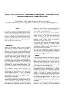
Figure 1: Geology map of the Study area 2.2 Data description and image enhancements Landsat 8, (OLI, year 2014) and Landsat 7, (ETM+, year 2000), scenes p168r060, p168r061 and p169r060 free of cloud cover for the year 2000 were downloaded from the USGS web site and preprocessed to reduce the effects of haze before mosaicing and subsetting. The image processing and 6

subsequent image enhancements are summarized by the methodology flow chart (Figure 2). First, standard PCA was performed on each of the images and the resulting covariance-variance matrix examined through factor loading as in Tables 1 and 2 for Landsat ETM+ and OLI, respectively. Factor Loading was to investigate the Principal Components (PCs) which contained the most information from geology band 7, and soil information from the red and SWIR bands 5 (in Landsat 7) and band 6 (in Landsat 8). This was the first step towards identifying components which enhanced lithology or lineaments that could be visualized in an FCC. From Tables 1 and 2, PC1 contained high geology and soil information, but positively correlated with other band information. Consequently, Independent Component Analysis (ICA) which performs better than PCA at separating class data was applied to obtain components with enhanced lineament and lithology information.

Pan-Band 8

Landsat 7 {pre-processed bands 1-5, and 7} OR Landsat 8 {pre-processed bands 1-7}

ICA

PCA and Factor loading Analysis

FCC (bands 573) FCC (bands 674)

Band ratioing and geology contrast criteria

Selection of PCs containing the most geologic information

IHS (FCC 573) IHS (FCC 674)

Advanced RGB clustering of FCC {3/2, 5/1, 7/4}/ FCC {4/2, 7/3, 6/5, }

RGB clustering of PCs (2,3,5)

Band ratio 5/1, 6/3

Application of non-directional filters

RGB clustering of PCs (2,4,5) Thresholding

Lineament visualization: FCC {IC1, PC5, Saturation band IHS 573} FCC {IC2, PC4, Saturation band IHS 674}

Density slicing

Extract lineaments Knowledge based classification

Band ratio geology classification

Overlay

PC soil classification map

Figure 2: Summary of the methodology flow chart using Landsat 7/ Landsat 8

Structural geology map

7

Table 1: PC Factor loading covariance-variance matrix, Landsat 7, Year 2000 Eigvec. 1 Eigvec 2 Eigvec 3 Eigvec 4 Eigvec 5 Eigvec 7 Var. contr. in %

PC1 0.35043 0.31187 0.40637 0.28295 0.58467 0.43920 96.64

PC2 0.14994 0.17774 -0.13773 0.82872 -0.13639 -0.47073 1.91

PC3 0.34351 0.41251 0.54636 -0.23965 -0.57760 -0.14922 1.18

PC4 -0.06653 -0.09581 0.35197 -0.24133 0.51478 -0.73436 0.17

PC5 0.41753 0.50378 -0.62644 -0.34225 0.19711 -0.15315 0.08

PC7 -0.74697 0.66182 0.03275 0.01907 0.04562 0.02273 0.02

Table 2: PC Factor loading covariance-variance matrix, Landsat 8, Year 2014 Eigvec. 1 Eigvec 2 Eigvec 3 Eigvec 4 Eigvec 5 Eigvec 6 Eigvec7 Var. contr. in %

PC1 0.24099 0.21217 0.21104 0.23250 0.58467 0.56277 0.37386 91.596

PC2 -0.05290 0.00164 0.03187 0.22847 -0.75238 0.37244 0.48909 6.840

PC3 -0.55771 -0.47775 -0.37807 -0.33049 0.21025 0.37243 0.16014 1.209

PC4 0.40784 0.20939 -0.09955 -0.62980 -0.20441 0.47883 -0.33498 0.208

PC5 -0.26256 -0.08576 0.14961 0.48878 -0.06988 0.42009 -0.69358 0.122

PC6 0.46573 -0.19418 -0.77211 0.38262 0.02520 0.00958 -0.04594 0.020

PC7 0.41942 -0.79864 0.42786 -0.05071 -0.02421 0.00558 0.00235 0.005

2.2.1 Image enhancement and knowledge based classification with Landsat 7 Following factor loading and band information in Table 1, PC2 was disqualified on the basis of high reflectance from vegetation in band 4, while PC3 and PC7 had a similar correlation between bands 5 and 7, complicating the differentiation of geology and soil information. PC1, PC4, and PC5 were therefore layer stack (as in Figure 2 (a)) and used for geology mapping with the help of IC1 (first independent component) to assist differentiate water features from rocks (Figure 2b). Knowledge based classification was applied using the following four components PC1, PC4, PC5 and IC1 where the classification boundary rules were defined (as in Table 3), according to colour information (from Figure 2a). Enquiry of the PC values in each channel was done at possible classes to establish class boundaries, which were consequently entered into the knowledge base engineer and saved. The Landsat subset images were then input, and the classification ran specifying the knowledge base engineer files. The boundaries were adjusted each time after a trial classification, until all the cells were classified. The result of the classification was 17 rock types and 3 water types discrimination.

8

(a)

(b)

Figure 2: FCC with (a) PC1, PC4, and PC5 (b) IC1, PC4, and PC5 Year 2000

9

Table 3: Knowledge based classification rules with PC1, PC4, PC5, IC1 components, for Landsat 7 Class Igneous rocks

Basic rocks Basalt Acidic Igneous

Granitoid gneiss

Intermediate igneous Intermediate (A.T.P) Ultra-basic Igneous

Pyroclastic unconsolid. Acidic metamorphic Basic metamorphic

Eulian unconsolidated

Fluvial Classic sediments

Organic unconsolid. Organic Limestone/Carbonates

Clear water Turbid water

Salty water

PC1 (0 – 559.738) 160 – 55 90 – 55 150 – 90 < 55 160 – 90 90 – 55 320 – 240 240 – 200 200 – 150 240 – 200 90 – 55 < 55 >320 320 – 260 260 – 200 260 – 240 320 – 240 240 – 160 260 – 200 200 – 160 240 –200 200 – 160 160 – 90 160 – 90 200 – 55 240 – 200 >320 320 - 240 >320 320 - 260 260 - 200 320 – 240 240 – 160 >320 320 - 240 >320 >320 320 – 240 >320 320 - 240 320 - 240 >320 320 – 240 200 – 90 200 – 90 > 320 320 – 260 >320 < 55 250 – 120 120 – 55 < 55 > 120 >240 320 - 240

PC4 (-96.16 – 44.33) 0 >5 >8 >5 20 – 0 >8 1 1.1 – 0.8 0.8 – 0.65 > 1.05 < 0.6 1 – 0.6 < 0.6 >1 < 0.6 1 – 0.6

7/3(0 – 7.91) 0.725 – 0.35 0.7 – 0.6 < 0.875 0.35 – 0.150 > 0.6 > 0.9 0.9 – 0.6 1.175 – 0.85 0.85 – 0.6 < 0.6 0.7 – 0.85 0.85 – 0.90 0.85 – 1.175 0.6 – 0.35 0.6 – 0.25 0.6 -0.35 > 0.85 0.85 – 0.6 > 1.175 1 – 0.5 > 1.175 0.7 -0.6 1 – 1.175 1.175 – 0.75 < 0.6 0.9 – 0.52 0.6 – 0.3 0.5 – 0.25 < 0.15 < 0.4 < 0.15 < 0.5 0.55 – 0.15 < 0.6

6/5(0 – 12.99) 0.75 – 0.5 0.75 – 0.35 < 0.65 < 0.5 0.75 – 0.25 < 0.75 > 0.75 > 0.9 > 0.75 > 0.5 0.35 – 0.85 0.4 – 0.75 1.35 – 0.95 < 0.65 0.9 – 0.5 < 0.5 0.95 – 0.75 > 0.85 > 0.75 0.95 – 0.25 > 0.8 0.85 – 0.75 0.95 – 0.25 0.75 – 1.0 < 0.5 > 0.85 > 0.75 0.825 – 0.5 3.9 >2 15

2.2.3 Image enhancement for lineament extraction and visualization Image enhancement for lineament extraction aimed at enhancing texture and increasing the possibilities of extracting structural linear features. Consequently, the implemented geology enhancing band ratios were examined individually for texture information, in which case band ratios 5/1 for Landsat 7 and 6/3 for Landsat 8 were found to have enhanced texture information compared to the other band ratios. Non-directional sober filter was applied on each band ratio followed by thresholding to select the significant lineament features. The same procedure was repeated using pan-band8 and the results merged into a single file; pan-band 8 and band ratio 5/1, Landsat 7 (Figure 6a), pan-band 8 and band ratio 6/3 Landsat 8 (Figure 6b).

Figure 6 (a): Lineament map using pan-band 8 and band ratio 5/1

16

Figure 6 (b): Lineament map using pan-band 8 and band ratio 6/3

Another method that was used to visualize the lineaments was the use of FCC with transformed feature components, in which PCA, ICA and IHS transformation were used. Firstly, a geology combination band (already identified as numerators in the band ratioing combinations, i.e. 5,7,3 for Landsat 7 and 6,7,4 for Landsat 8), was transformed from Red Green Blue (RGB) space to IHS (Intensity, Hue saturation) space. Secondly, a new RGB was formed with an IC, PC and Saturation component as the Red, Green and Blue channels respectively. The IC and PC were identified through PC Factor loading, those which contained most geology information. A variation of visualizing lineament alone was done using an RGB combination of the edges obtained from band ratio, band 8 and slope in the Blue channel.

17

3. RESULTS AND DISCUSSIONS The results consist of comparisons: firstly, for Landsat 7, comparison between classifications with band ratios; secondly, for each Landsat dataset, comparison between the PC and band ratio enhanced classification; thirdly, comparison between Landsat 7 and 8 geology classifications and then visualization. Figures 7 and 8 were the classified geological maps obtained from band ratio sets (3/2, 5/1, 7/4, 5/4, and 7/3) and (3/2, 5/1, 7/3, 5/4), respectively. Comparing Figures 7 and 8, more rock discrimination was achieved in Figure 7, which had more band ratios. The extra band ratio 7/4 was included in Figure 7 classification using a multiplicative band, 7/3*7/4.

Figure 7: Geology classification map using band ratios 3/2, 5/1, 7/4, 5/4, 7/3

18

Figure 8: Geology classification map using band ratios 3/2, 5/1, 7/3

Geology contrast by band ratios was facilitated by the use of bands from different spectral regions, avoiding band redundancy and use of geology enhancing bands as numerators in the ratio combination. Further, each individual band ratio work to emphasize certain minerals in a rock i.e. 3/2- iron oxides, 5/4- ferrous minerals, 5/1-variation of soil line, 7/3 & 7/4 – geology components. Thus, better discrimination ability was afforded with the combination 3/2, 5/1, 7/4 (containing unique bands), compared to the combination 3/2, 5/1, 7/3 (which had band 3 redundancy). It was noted that although the use of multiplicative bands introduced redundancy, its use resulting to square of a band in the numerator or dominator of a band ratio, e.g. 7/3*7/4 or 5/4*7/4, yielded enhanced contrast (e.g. Figure 3 b & c) unlike multiplicative bands with cancelling effects, e.g. (7/3*3/2) or completely different (7/3*5/4). Thus, the inclusion of band ratio 7/4 into the classification (Figure 7), yielded increased discrimination of rock types. 19

On the other hand, geological mapping with Landsat 7, PCs (1, 4, 5) and IC1 (Figure 9), resulted in slightly increased rock discrimination and failure to detect water clay minerals. This could be explained using Figures 2, whereby the inclusion of IC1 into the PCs-FCC had better visual discrimination of rock from water covers. Also, PC being a feature reduction method, led to merging geological information, thus the selected PCs contained most of the needed information. However, comparing the FCC of the PCs versus band ratios, band ratios had better visual contrast enhancement. Consequently, it was much easier to implement density slicing (set class boundaries) with band ratios-FCC as compared to PC-FCC.

Figure 9: Geology classification map using PCs 1, 4, 5 and IC1

The use of band ratios with the Landsat 8 dataset, differed slightly owing to an extra band 6 in the Shortwave Infrared Region (SWIR) and the far visible band 1 which is lacking in Landsat 7 bands. Consequently, the geology enhancing bands were 6, 7, 4, corresponding to Landsat 7 bands 5, 7, 3. 20

Observing geology band ratio rule by Drury (1993), a combination comprising ratios 4/2, 7/3, 6/5 (see, Figure 5a) was found to have the most geology contrast and the inputs were implemented in a classification resulting in Figure 10. In this scenario, the use of multiplicative band, 7/3*7/4 did not yield significant contrast improvement (see, Figure 5b) and consequently, band ratio 7/4 was not used in the classification. It was noted that the inability to utilise all the bands in the visible region affected water discrimination ability; even with the attempt to use IC1 together with band ratios in the classification. However, with only the 3 band ratios, more geology features were mapped compared to all Landsat 7 with band ratios (Figure 7). This may be attributed to the extra band in the SWIR (band 6) region of Landsat 8, and the narrower bandwidth spectral bands of Landsat 8 compared to Landsat 7.

21

Figure 10: Geology classification map using band ratios (4/2, 7/3, 6/5) Landsat 8

On the other hand, geological classification with Landsat 8, PCs 2,4,5,3 and IC1 was mapped in Figure 11. In comparison with Landsat 8 band ratio classification (Figure 10), similar numbers of rock types are discriminated with both classifications. However, band ratios classification with Landsat 8 achieved water clay deposits which were not mapped in the PCs classification. This observation was similar to Landsat 7 classified geological maps. Also, similar to Landsat 7, it was easier to implement density slicing with band ratios-FCC compared to PCs-FCC.

Figure 11: Geology classification map using PCs 2,4,5,3 and IC1, Landsat 8

Representation of structural geology was completed with both lineament and lithology mapping for both Landsat sets with the band ratios maps overlaid with lineament maps extracted with the application of non directional filters and thresholding. The criteria for the choice of band ratios 5/1 and 6/3 for Landsat 7 and 8 respectively, was based on enhanced texture qualities, while the use of pan-band 8 was aimed at increasing the number of lineaments due to its higher spatial resolution. However, it was observed that while Landsat 8, pan-band 8 spans only the visible region compared 22

to Landsat 7, spanning Red, green and NIR regions of the spectrum, Landsat 8 band 8 edges had more noise even after thresholding unlike Landsat 7 band 8 edges, which appeared more sharp. The edges obtained from band ratios 5/1 and 6/3 for Landsat 7 and 8 respectively, complemented the missing lineament features in pan-band 8. Although, both pan-bands 8 from Landsat 7 and 8 were properly matched, it was not possible to substitute them because the time epoch (years 2000 and 2014) was large and contained some discernable changes in feature outlines. The resulting structural geology from the overlay between the classified geology maps and the lineaments were Figures 12 and 13 for Landsat 7 and 8 respectively, which had an added texture component to the lithology maps.

Figure 12: Structural geology band ratio classification map with Landsat 7

23

Figure 13: Structural geology band ratio classification maps with Landsat 8

Another variation of visualizing the lineaments alone was presented in Figure 14 (a) and (b) in shaded relief maps comprising RGB of the edges extracted from band ratio (5/1 for Landsat 7, 6/3 for Landsat 8), pan-band8 and slope map. The folds and fault lines along the Rift Valley floor and drainage channels in the study area were more enhanced in this representation compared to Figures 15 (a) and (b). Figures 15 revealed enhanced rock discrimination as well as lineament visualization and were comprised of: Figure 15 (a) IC1, PC5 and Saturation band (IHS transformation of bands 5,7,3) of Landsat 7; Figure 15 (b) IC1, PC4, and Saturation band (IHS transformation of bands 6,7,4) of Landsat 8. This idea was advanced from works by Mondini et al. (2011) who mapped 24

landslides using a multi-change detection technique involving an FCC comprising: change in NDVI, IC4 and PC4 using Formasat images. While extending this idea, the authors of this paper have advanced the idea to map landslide scars in the study area, by detecting exposed geological features in a recent publication (Mwaniki et al., 2015b).

(a)

(b)

Figure 14: (a) RGB with edges from Band ratio 5/1, Band 8 & Slope (b) RGB with edges from Band ratio 6/3, Band 8 & Slope

(a)

(b)

Figure 15(a): FCC {IC1,PC5, Saturation Band (5,7,3)} Landsat 7

(b): FCC {IC1,PC4, Saturation Band (6,7,4)} Landsat 8 25

4. CONCLUSIONS It was noted that more geology contrast was achieved with band ratioing compared to the use of PCs for both Landsat datasets. While PC geological classification may offer an alternative to the use of band ratios, its success depend mainly on the PC Factor-loading and further, the use of feature transform with ICA components. On the other hand, the success of band ratios in geological mapping with Landsat datasets, was the increased contrast with band ratio combinations utilising different spectral regions and following Drury’s geological rule (Drury, 1993). In addition to this rule, this research has also established that more contrast is enhanced with vegetation enhancing bands as denominators in the band ratios, use of geology and soil information containing bands as numerators and the avoidance of band redundancy in the band ratio combination. The more band ratios were used, the more the discrimination against many rock types. However, Landsat 8 achieved more rock discrimination than Landsat 7, even with the same number of band ratios, a factor that was attributed to its narrower bands and the extra SWIR band 6 which is more sensitive to geology compared to Landsat 7, band 5. It was found that although pan-band 8 (with higher spatial resolution) yields more detailed lineament features, in vegetated areas it had completely no lineament information which could be attributed to the fact that it covers the lower spectral region of the spectrum. Particularly Landsat 8, band 8 lineaments had more noise compared to Landsat 7, band 8 lineaments which appeared clearer and sharper. This was explained by the slight difference in the span of the spectral region occupied by the two datasets i.e. only visible region for Landsat 8 but both visible and NIR regions for Landsat 7. Instead, band ratios involving SWIR and visible regions of the spectrum (i.e. band ratios 5/1 and 6/3 for Landsat 7 and 8 respectively) were found to have more texture and complemented lineaments from pan-band 8. The use of FCC with enhanced components comprising an IC, PC and saturation band of the RGB bands contributing most to enhance geology, was explored to enhance geology and lineament visualisation. The result was superior compared to the use of PC only FCC, a strength derived from the combination of bands from different spectral regions; combinations (5, 7, 3) for Landsat 7 and (6, 7, 4) Landsat 8. The use of band ratios was limited to the few ratios enhancing texture and therefore, lineaments could only be visualised separately after filter and thresholding, or enhanced shaded relief with slope or overlaid to the classified geology maps.

26

ACKNOWLEDGEMENTS The author wishes to thank John G. Mbaka for the assistance with proof-reading and all the other anonymous reviewers who have ensured the quality of this paper is improved. Also, the continued support of the Jomo Kenyatta University of Technology and Agriculture is highly appreciated. REFERENCES Abdeen, M. M., & Abdelghaffar, A. A. (2008). Mapping Neoproterozoic structures along the central Allaqiheiani suture, Southeastern Eqypt, using remote sensing and field data (Vol. 3). Presented at the 29th Asian Conference on Remote Sensing, Colombo, Sri Lanka: Curran Associates, Inc. Retrieved from http://www.a-a-r-s.org/acrs/proceeding/ACRS2008/Papers/TS%2036.1.pdf Abdeen, M. M., Thrurmond, K. A., Abdelsalam, G. M., & Stern, J. R. (2001, November). Application of ASTER Band-ratio Images for Geological Mapping in Arid Regions: The Neoproterozoic Allaqi Suture, Egypt. Presented at the Geological Society of America Annual Meeting, Boston, USA. Retrieved from https://gsa.confex.com/gsa/2001AM/finalprogram/abstract_27348.htm Abdullah, A., Nassr, S., & Ghaleeb, A. (2013). Remote Sensing and Geographic Information System for Fault Segments Mapping a Study from Taiz Area, Yemen. Journal of Geological Research, 2013, 1–16. http://doi.org/10.1155/2013/201757 Ali, E. A., El Khidir, S. O., Babikir, A. A., & Abdelrahnam, E. M. (2012). Landsat ETM+7 Digital Image Processing Techniques for Lithological and Structural Lineament Enhancement: Case Study Around Abidiya Area, Sudan. The Open Remote Sensing Journal, 5(1), 83–89. http://doi.org/10.2174/1875413901205010083 Argialas, D., Mavrantza, O., & Stefouli, M. (2003). Automatic mapping of tectonic lineaments (faults) using methods and techniques of Photointerpretation /Digital Remote Sensing and Expert Systems (Geology No. THALES Project 1174). Aspinall, R. J., Marcus, W. A., & Boardman, J. W. (2002). Considerations in collecting, processing, and analysing high spatial resolution hyperspectral data for environmental investigations. Journal of Geographical Systems, 4(1), 15–29. http://doi.org/10.1007/s101090100071 Binaghi, E., Madella, P., Grazia Montesano, M., & Rampini, A. (1997). Fuzzy contextual classification of multisource remote sensing images. IEEE Transactions on Geoscience and Remote Sensing, 35(2), 326–340. http://doi.org/10.1109/36.563272 Boettinger, J. L., Ramsey, R. D., Bodily, J. M., Cole, N. J., Kienast-Brown, S., Nield, S. J., … Stum, A. K. (2008). Landsat Spectral Data for Digital Soil Mapping. In A. E. Hartemink, A. McBratney, & M. de L. Mendonça-Santos (Eds.), Digital Soil Mapping with Limited Data (Vol. III, pp. 193–202). Dordrecht: Springer Netherlands. Campbell, J. B. (2002). Band ratios. In Introduction to remote sensing (3rd ed., p. 505). New York: Guilford Press. Campbell, J. B. (2009). Remote sensing of Soils. In The Sage handbook of remote sensing (pp. 341–354). Thousand Oaks, CA: Sage. Carranza, E. J. M., & Hale, M. (2002). Mineral imaging with Landsat Thematic Mapper data for hydrothermal alteration mapping in heavily vegetated terrane. International Journal of Remote Sensing, 23(22), 4827–4852. http://doi.org/10.1080/01431160110115014

27

Chaabouni, R., Bouaziz, S., Peresson, H., & Wolfgang, J. (2012). Lineament analysis of South Jenein Area (Southern Tunisia) using remote sensing data and geographic information system. The Egyptian Journal of Remote Sensing and Space Science, 15(2), 197–206. http://doi.org/10.1016/j.ejrs.2012.11.001 Chen, X., & Campagna, D. J. (2009). Remote Sensing of Geology. In The Sage handbook of remote sensing (pp. 328–340). Thousand Oaks, CA: Sage. Cloutis, E. A. (1996). Review Article Hyperspectral geological remote sensing: evaluation of analytical techniques. International Journal of Remote Sensing, 17(12), 2215–2242. http://doi.org/10.1080/01431169608948770 Cortez, L., Durão, F., & Ramos, V. (1997). Testing some Connectionist Approaches for Thematic Mapping of Rural Areas. In I. Kanellopoulos, G. G. Wilkinson, F. Roli, & J. Austin (Eds.), Neurocomputation in Remote Sensing Data Analysis (pp. 142–150). Berlin, Heidelberg: Springer Berlin Heidelberg. Retrieved from http://link.springer.com/10.1007/978-3-642-59041-2_16 Cudahy, T. J., Hewson, R., Huntington, J. F., Quigley, M. A., & Barry, P. S. (2001). The performance of the satellite-borne Hyperion hyperspectral VNIR-SWIR imaging system for mineral mapping at Mount Fitton, South Australia (Vol. 1, pp. 314–316). IEEE. http://doi.org/10.1109/IGARSS.2001.976142 Drury, S. A. (1993). Image interpretation in geology (2nd ed). London ; New York: Chapman & Hall. Retrieved from http://library.dmr.go.th/library/TextBooks/10146.pdf Favretto, A., Geletti, R., & Civile, D. (2013). Remote sensing as a preliminary analysis for the detection of active tectonic structures: an application to the Albanian orogenic system. Geoadria, 18(2), 97–111. Gad, S., & Kusky, T. (2006). Lithological mapping in the Eastern Desert of Egypt, the Barramiya area, using Landsat thematic mapper (TM). Journal of African Earth Sciences, 44(2), 196–202. http://doi.org/10.1016/j.jafrearsci.2005.10.014 Gong, P. (1996). Integrated Analysis of Spatial Data from Multiple sources: Using Evidential reasoning and Artificial Neural network Techniques for Geological mapping. Photogrammetric Engineering and Remote Sensing, 62(5), 513–523. Govender, M., Chetty, K., & Bulcock, H. (2007). A review of hyperspectral remote sensing and its application in vegetation and water resource studies. Water SA, 33(2), 145–152. http://doi.org/10.4314/wsa.v33i2.49049 Gupta, R. P. (2013). Remote Sensing Geology. Berlin, Heidelberg: Springer Berlin Heidelberg. Retrieved from http://dx.doi.org/10.1007/978-3-662-12914-2 Harris, J. R., Eddy, B., Rencz, A., de Kemp, E., Budketwitsch, P., & Peshko, M. (2001). Remote sensing as a geological mapping tool in the Arctic: preliminary results from Baffin Island, Nunavut, 2001-E12, 13. Hung, L. Q., Batelaan, O., & De Smedt, F. (2005). Lineament extraction and analysis, comparison of LANDSAT ETM and ASTER imagery. Case study: Suoimuoi tropical karst catchment, Vietnam. In M. Ehlers & U. Michel (Eds.), Proceedings of SPIE Remote sensing for Environmental monitoring, GIS applications and Geology (Vol. 5983, p. 59830T–59830T–12). International Society for Optics and Photonics. http://doi.org/10.1117/12.627699 Jolliffe, I. (2005). Principal Component Analysis (2nd ed.). John Wiley & Sons, Ltd. Karnieli, A., Meisels, A., Fisher, L., & Arkin, Y. (1996). Automatic Extraction and Evaluation of Geological Linear features from Digital Remote Sensing Data Using a Hough Transform. Photogrammetric Engineering and Remote Sensing, 62(5), 525–531. 28

Kavak, K. S. (2005). Determination of palaeotectonic and neotectonic features around the Menderes Massif and the Gediz Graben (West. Turkey) using Landsat TM image. International Journal of Remote Sensing, 26(1), 59–78. http://doi.org/10.1080/01431160410001709994 Kenea, N. H. (1997). Improved geological mapping using Landsat TM data, Southern Red Sea Hills, Sudan: PC and IHS decorrelation stretching. International Journal of Remote Sensing, 18(6), 1233–1244. http://doi.org/10.1080/014311697218386 King, T. V. V., Kokaly, R. F., Hoefen, T. M., & Johnson, M. R. (2012). Hyperspectral remote sensing data maps minerals in Afghanistan. Eos, Transactions American Geophysical Union, 93(34), 325. http://doi.org/10.1029/2012EO340002 Kocal, A., Duzgun, H. S., & Karpuz, C. (2004). Discontinuity mapping with automatic lineament extraction from high resolution satellite imagery. In Proceedings of the XXth ISPRS Congress. Istanbul, Turkey. Retrieved from http://www.cartesia.org/geodoc/isprs2004/comm7/papers/205.pdf Kruse, A. F. (1998). Advances in Hyperspectral Remote Sensing for Geologic Mapping and Exploration. In 9th Australasian Remote Sensing Conference. Sydney, Australia. Retrieved from http://www.hgimaging.com/PDF/Kruse_9th_australasian_rs_98.pdf Laake, A. (2011). Integration of satellite Imagery, Geology and geophysical Data. In Earth and Environmental Sciences (pp. 467–492). INTECH Open Access Publisher. Retrieved from http://cdn.intechopen.com/pdfs/24568.pdf Maina-Gichaba, C., Kipseba, E. K., & Masibo, M. (2013). Overview of Landslide Occurrences in Kenya. In Developments in Earth Surface Processes (Vol. 16, pp. 293–314). Elsevier. Retrieved from http://erepository.uonbi.ac.ke/bitstream/handle/11295/66302/Full%20text.pdf?sequence=1 Marghany, M. (2012). Three-dimensional lineament visualization using fuzzy B-spline algorithm from multispectral satellite data. In B. Escalante-Ramirez (Ed.), Remote Sensing - advanced techniques and platforms (pp. 213–232). Croatia: INTECH Open Access Publisher, University Campus STeP Ri. Marghany, M., & Hashim, M. (2010). Lineament Mapping Using Multispectral Remote Sensing Satellite Data. Research Journal of Applied Sciences, 5(2), 126–130. http://doi.org/10.3923/rjasci.2010.126.130 Mavrantza, O. D., & Argialas, D. P. (2006). Object-oriented image analysis for the identification of geologic lineaments. International Archives of Photogrammetry, Remote Sensing and Spatial Information Sciences, 36(4). Mia, B., & Fujimitsu, Y. (2012). Mapping hydrothermal altered mineral deposits using Landsat 7 ETM+ image in and around Kuju volcano, Kyushu, Japan. Journal of Earth System Science, 121(4), 1049–1057. http://doi.org/10.1007/s12040-012-0211-9 Mwaniki, M. W., Matthias, M. S., & Schellmann, G. (2015). Application of Remote Sensing Technologies to Map the Structural Geology of Central Region of Kenya. IEEE Journal of Selected Topics in Applied Earth Observations and Remote Sensing, 8(4), 1855–1867. http://doi.org/10.1109/JSTARS.2015.2395094 Mwaniki, M. W., Ngigi, T. G., & Waithaka, E. H. (2011). Rainfall Induced Landslide Probability Mapping for Central Province. In Fourth International Summer School and Conference (Vol. 1, 2011, pp. 203–213). JKUAT, Kenya: Publications of AGSE Karlsruhe, Germany. http://doi.org/10.13140/RG.2.1.4509.9046 Ngecu, W. M., & Mathu, E. M. (1999). The El-Nino- triggered landslides and their socio-economic impact on Kenya. Engineering Geology, 38(4), 277–285.

29

Ngecu, W. M., Nyamai, C. M., & Erima, G. (2004). The extent and significance of mass-movements in Eastern Africa: case studies of some major landslides in Uganda and Kenya. Environmental Geology, 46(8), 1123–1133. http://doi.org/10.1007/s00254-004-1116-y Ninomiya, Y., Fu, B., & Cudahy, T. J. (2005). Detecting lithology with Advanced Spaceborne Thermal Emission and Reflection Radiometer (ASTER) multispectral thermal infrared ‘radiance-at-sensor’ data. Remote Sensing of Environment, 99(1–2), 127–139. http://doi.org/10.1016/j.rse.2005.06.009 Novak, I. D., & Soulakellis, N. (2000). Identifying geomorphic features using Landsat-5/TM data processing techniques on Lesvos, Greece. Geomorphology, 34(1–2), 101–109. http://doi.org/10.1016/S0169555X(00)00003-9 Ogallo, S. N., Gaya, C. O., & Omuterema, S. O. (2006). Landslide Hazard Zonation Mapping for Murang’a District, Kenya. In Proceedings of the 1st International Conference on Disaster Management & Human Security in Africa (pp. 303–308). Masinde Muliro University of Science & Technology, Kakamega, Kenya: Center for Disaster Management & Humanitarian Assisstance. Ott, N., Kollersberger, T., & Tassara, A. (2006). GIS analyses and favorability mapping of optimized satellite data in northern Chile to improve exploration for copper mineral deposits. Geosphere, 2(4), 236. http://doi.org/10.1130/GES00017.1 Pal, S. K., Majumdar, T. J., & Bhattacharya, A. K. (2007). ERS-2 SAR and IRS-1C LISS III data fusion: A PCA approach to improve remote sensing based geological interpretation. ISPRS Journal of Photogrammetry and Remote Sensing, 61(5), 281–297. http://doi.org/10.1016/j.isprsjprs.2006.10.001 Papadaki, E. S., Mertikas, S. P., & Sarris, A. (2011). Identification of lineaments with possible structural origin using ASTER images and DEM derived products in Western Crete, Greece. In EARSeL ePrcoceedings 10 (pp. 9–26). Retrieved from http://eproceedings.org/static/vol10_1/10_1_papadaki1.pdf Perez, F. G., Higgins, C. T., & Real, C. R. (2006). Evaluation of use of remote sensing imagery in refinement of geological mapping for seismic hazard zoning in northern loss angeles county, California. In Proceedings of ISPRS XXXVI Congress (Vol. XXXVI Part 7). Retrieved from http://www.isprs.org/proceedings/xxxvi/part7/PDF/180.pdf Pour, A. B., & Hashim, M. (2013). Fusing ASTER, ALI and Hyperion data for enhanced mineral mapping. International Journal of Image and Data Fusion, 4(2), 126–145. http://doi.org/10.1080/19479832.2012.753115 Prost, L. G. (2001). Remote sensing for geologists: a guide to image interpretation. [Amsterdam]; New York; Abingdon: Gordon & Breach ; Marston. Qari, M. H. T., Madani, A. A., Matsah, M. I. M., & Hamimi, Z. (2008). Utilization of Aster and Landsat data in geologic mapping of basement rocks of Arafat area, Saudi Arabia. The Arabian Journal for Science and Engineering, 33(1C), 99–117. Rahman, M. M., Tetuko Sri Sumantyo, J., & Sadek, M. F. (2010). Microwave and optical image fusion for surface and sub-surface feature mapping in Eastern Sahara. International Journal of Remote Sensing, 31(20), 5465–5480. http://doi.org/10.1080/01431160903302999 Rahnama, M., & Gloaguen, R. (2014). TecLines: A MATLAB-Based Toolbox for Tectonic Lineament Analysis from Satellite Images and DEMs, Part 1: Line Segment Detection and Extraction. Remote Sensing, 6(7), 5938–5958. http://doi.org/10.3390/rs6075938

30

Rajendran, S., Thirunavukkaraasu, A., Poovalingaganesh, B., Kumar, K. V., & Bhaskaran, G. (2007). Discrimination of low-grade magnetite ores using remote sensing techniques. Journal of the Indian Society of Remote Sensing, 35(2), 153–162. http://doi.org/10.1007/BF02990779 Ramli, M. F., Yusof, N., Yusoff, M. K., Juahir, H., & Shafri, H. Z. M. (2010). Lineament mapping and its application in landslide hazard assessment: a review. Bulletin of Engineering Geology and the Environment, 69(2), 215–233. http://doi.org/10.1007/s10064-009-0255-5 Rigol-Sanchez, J. P., Chica-Olmo, M., & Abarca-Hernandez, F. (2003). Artificial neural networks as a tool for mineral potential mapping with GIS. International Journal of Remote Sensing, 24(5), 1151–1156. http://doi.org/10.1080/0143116021000031791 Roy, D. P., Wulder, M. A., Loveland, T. R., C.E., W., Allen, R. G., Anderson, M. C., … Zhu, Z. (2014). Landsat-8: Science and product vision for terrestrial global change research. Remote Sensing of Environment, 145, 154–172. http://doi.org/10.1016/j.rse.2014.02.001 Sabins, F. F. (1997). Remote sensing: principles and interpretation. New York: W.H. Freeman and Company. Sabins, F. F. (1999). Remote sensing for mineral exploration. Ore Geology Reviews, 14(3), 157–183. http://doi.org/10.1016/S0169-1368(99)00007-4 Sultan, M., Arvidson, R. E., Sturchio, N. C., & Guinness, E. A. (1987). Lithologic mapping in arid regions with Landsat thematic mapper data: Meatiq dome, Egypt. Geological Society of America Bulletin, 99(6), 748. http://doi.org/10.1130/0016-7606(1987)992.0.CO;2 Suzen, M. L., & Toprak, V. (1998). Filtering of satellite images in geological lineament analyses: An application to a fault zone in Central Turkey. International Journal of Remote Sensing, 19(6), 1101–1114. http://doi.org/10.1080/014311698215621 Ultsch, A., Korus, D., & Wehrmann, A. (1995). Neural networks and their rules for classification in marine geology. In Raum und zeit in Umweltinformationsystemen (Vol. 7, pp. 676–693). Marburg: Metropolis. van der Meer, F. D., van der Werff, H. M. A., van Ruitenbeek, F. J. A., Hecker, C. A., Bakker, W. H., Noomen, M. F., … Woldai, T. (2012). Multi- and hyperspectral geologic remote sensing: A review. International Journal of Applied Earth Observation and Geoinformation, 14(1), 112–128. http://doi.org/10.1016/j.jag.2011.08.002 Wahid, M., & Ahmed, R. E. (2006). Identifying Geomporphic Features between Ras Gemsha and Safaga, Red Sea Coast, Egypt, Using Remote Sensing Techniques. Marine Geology, 17(1), 23. Zhu, A.-X., Wang, R., Qiao, J., Qin, C.-Z., Chen, Y., Liu, J., … Zhu, T. (2014). An expert knowledge-based approach to landslide susceptibility mapping using GIS and fuzzy logic. Geomorphology, 214, 128–138. http://doi.org/10.1016/j.geomorph.2014.02.003

31