Geometric Semantic Genetic Programming is Overkill

Geometric Semantic Genetic Programming is Overkill? Tomasz P. Pawlak Institute of Computing Science, Poznan University of Technology [email protected]

Abstract Recently, a new notion of Geometric Semantic Genetic Programming emerged in the field of automatic program induction from examples. Given that the induction problem is stated by means of function learning and a fitness function is a metric, GSGP uses geometry of solution space to search for the optimal program. We demonstrate that a program constructed by GSGP is indeed a linear combination of random parts. We also show that this type of program can be constructed in a predetermined time by much simpler algorithm and with guarantee of solving the induction problem optimally. We experimentally compare the proposed algorithm to GSGP on a set of symbolic regression, Boolean function synthesis and classifier induction problems. The proposed algorithm is superior to GSGP in terms of training-set fitness, size of produced programs and computational cost, and generalizes on test-set similarly to GSGP.

1

Introduction

Recently in the field of automatic program induction from examples, a new branch of Genetic Programming (GP) called Geometric Semantic Genetic Programming (GSGP) [18] arose. GSGP involves program semantics, meant as a vector of program outcomes produced in the effect of its execution on the given sample program inputs (fitness cases). The key idea behind GSGP is to define fitness function by means of a metric, where the first metric argument is semantics of a program under assessment and the second one is the optimal target semantics. This formulation causes fitness landscape to take shape of a cone, with the target semantics in the apex [27,24,26]. GSGP uses specialized search operators that utilize this conic shape to efficiently search the program space. Theoretical analyses have showed that each application of the geometric operators is characterized by beneficial expected improvement of fitness [17] and guaranteed pessimistic bound on change of fitness [26]. Nevertheless, GSGP has crucial design drawback that causes each offspring to be bigger than its parent(s). GSGP crossover leads to exponential growth and GSGP mutation to linear growth of programs over the course of evolution. ?

The final publication is available at Springer via https://doi.org/10.1007/ 978-3-319-30668-1_16.

The size of the produced programs may put the use of GSGP in real world applications under a question. This state of affairs changed, when Castelli et al. [2] proposed graph-like encoding of tree programs to efficiently store overgrowth programs in memory. This allowed use of GSGP in many real-world applications [2,4,3,15,30,31], however the obtained programs are still oversized. We demonstrate that a final program produced by GSGP implements, indeed, a linear combination of programs from the initial population, i.e., can be considered as an linear combination of random parts. We show that qualitatively equivalent results can be achieved by much simpler means than GP. We address all three problem domains, for which GSGP was designed: symbolic regression, Boolean function synthesis and classifier induction [18]. We propose an exact algorithm, that guarantees reaching the optimum, in opposition to GSGP, which as a stochastic metaheuristics does not guarantee this. What is more, the exact algorithm produces smaller programs and in shorter time than GSGP.

2

Problem statement and solution in Geometric Semantic Genetic Programming

A program p ∈ P is a function that maps a set of inputs I into a set of outputs O, which we denote by o = p(in), where in ∈ I and o ∈ O. We consider only deterministic programs that feature no side effects, nor memory persistent across executions. Semantics s ∈ S is a vector s = [o1 , o2 , ..., on ], where ∀oi ∈ O and S is a semantic space (a vector space). Semantic mapping is a function s : P → S, with property s(p1 ) = s(p2 ) ⇐⇒ ∀i p1 (ini ) = p2 (ini ). In other words, semantics s(p) of a program p is a vector of p’s outputs when executed on a fixed set of inputs I ⊂ I, i.e., s(p) = [p(in1 ), p(in2 ), ..., p(inn )], ini ∈ I. In GSGP program induction problem Π = (t, f ) is an optimization problem, where t is the target semantics, and f is a metric, such that f (p) = kt, s(p)k. The aim of program induction problem is to synthesize program p∗ , which semantics equals t, i.e., t = s(p∗ ) and f (p∗ ) = 0. Note that Π is stated in terms of learning function h : I → O. GSGP attempts to solve the abovementioned problem by initializing population of random programs, e.g., using ramped half-and-half [9], then iteratively searches the program space using geometric operators defined below (definitions come from [18]). Definition 1. Given a parent program p, r-geometric mutation is an operator that produces offspring p0 in a ball of radius r centered in p, i.e., ks(p), s(p0 )k ≤ r. Definition 2. (Algorithms for geometric mutation) Symbolic regression: Given parent arithmetic program p, an offspring is a program p0 = p + r · (m1 − m2 ), where m1 and m2 are random arithmetic programs that output values in range [0, 1]. Boolean: Given Boolean parent program p, an offspring is a program p0 = m ∨ p with probability 0.5, p0 = m ∧ p otherwise, where m is a random minterm. Classifier: Given parent classifier p, an offspring is a program

p0 = IF cond T HEN c ELSE p, where cond is a random condition that is true only for a single combination of attributes and c ∈ O is a random class. Definition 3. Given parent programs p1 , p2 , geometric crossover is an operator that produces offspring p0 in a segment between p1 and p2 , i.e., ks(p1 ), s(p2 )k = ks(p1 ), s(p0 )k + ks(p0 ), s(p2 )k. Definition 4. (Algorithms for geometric crossover) Symbolic regression: Given parent arithmetic programs p1 , p2 , an offspring is a program p0 = mp1 +(1−m)p2 , where m is a function that returns values in range [0, 1]. Boolean: Given Boolean parent programs p1 , p2 , an offspring is a program p0 = (p1 ∧ m) ∨ (m ∧ p2 ), where m is a random Boolean program. Classifier: Given parent classifiers p1 , p2 , an offspring is a program p0 = IF cond T HEN p1 ELSE p2 , where cond is a random condition. In the essence geometric operators conduct linear transformation of parents, which we formalize below: Definition 5. A linear combination over a field is an expression of elements from this field multiplied by constants and added together. Symbolic regression: Field elements are real numbers; + (arithmetic addition) and · (arithmetic multiplication) meet axioms of addition and multiplication, respectively. Boolean: (GF (2) field) Field elements are 0 and 1; ⊕ (xor) and ∧ (and) meet axioms of addition and multiplication, respectively. Classifier: Field elements are Boolean 0 and 1, classes c1 , c2 , ... and null  (no decision); 6 and 7 meet axioms of addition and multiplication, respectively. IF is composition of 6 and 7: IF cond T HEN c1 ELSE c2 ≡ cond 7 c1 6 cond 7 c2 .1 Lemma 1. An offspring p0 obtained from parent p using r-geometric mutation is a linear combination of p and an other random program. Proof. The proof comes from Definition 2, each offspring’s formula combines p with other parts using only addition and/or multiplication by a constant (e.g., weight). Symbolic regression: p0 is addition of p and program r · (m1 − m2 ). Boolean: by expanding p0 = m ∨ p to p0 = m ⊕ p ⊕ m ∧ p, p0 is addition of p, m and program m ∧ p, or by transforming p0 = m ∧ p to p0 = p ⊕ m ∧ p, p0 is addition of p and a program m ∧ p. Classifier: IF term is a weighted addition of c and p, where respective weights for c and p are either 0 and 1, or 1 and 0, depending on cond’s Boolean value. Lemma 2. An offspring p0 obtained from parents p1 and p2 using geometric crossover is a linear combination of p1 and p2 . 1

6 for two Booleans is equivalent to ∨, for two classes outputs the one with lower id, for a class and  outputs this class, otherwise . 7 for two Booleans is equivalent to ∧, for two classes outputs the one with greater id, for 1 and a class outputs this class, otherwise . We omitted full tables of these functions for brevity.

Proof. Proof comes from Definition 4, each offspring’s formula combines p1 and p2 with other parts using only addition and/or multiplication by a constant (e.g., weight). Symbolic regression: p0 is weighted addition of p1 and p2 , where m and (1 − m) are weights. Boolean: by transforming p0 = (p1 ∧ m) ∨ (m ∧ p2 ) to p0 = (p1 ∧ m) ⊕ (m ∧ p2 ), p0 is weighted addition of p1 and p2 , where m and m are weights. Classifier: IF term is a weighted addition of p1 and p2 , where respective weights for c and p are either 0 and 1, or 1 and 0, depending on cond’s Boolean value. Theorem 1. A program produced by GSGP in any generation after the initial one is a linear combination of programs from the initial population and other random programs. Proof. Let Pg denote population and Mg set of random functions added by geometric operators in generation g ∈ N≥1 . Proof by induction: each program p2 ∈ P2 is linear combination of programs p1 ∈ P1 and m1 ∈ M1 by Lemmas 1 and 2. A program pi ∈ Pi is a linear combination of programs pi−1 ∈ Pi−1 and random programs mi−1 ∈ Mi−1 . By commutativity of linear combinations each program in Pi is a linear combination of programs in P1 and M1 , M2 , .., Mi−1 . This leads to the straightforward conclusion that if the initial population consists of randomly generated programs, e.g., using ramped half-and-half [9], in the essence a program produced by GSGP is a linear combination of random parts. However, linear combination of, or even interpolation2 using random parts can be done analytically with guarantee of constructing the optimal program p∗ .

3

Function learning using linear combination

In this section, we show how to interpolate points from different semantic spaces: Rn , {0, 1}n and {c1 , c2 , ..., ck }n to obtain the optimal program p∗ . To interpolate given function h : I → O using random program parts, two conditions have to be met: 1. Set of semantics S of random program parts must be linearly independent, 2. Target t must be expressible by linear combination of semantics from S. The first condition is there, because the set of semantics that can be expressed by linearly combining the semantics from S is exactly the same like for S with linearly dependent semantics discarded. The second condition is the necessary one to solve the program induction problem Π. The above conditions can be met by making S a basis of semantic space S. Below, we present Linear Combination (LC) algorithm. Although the general idea behind LC is maintained across domains, a particular realization is domaindependent. For each domain, we divide the presentation of LC into two parts: 2

The distinction between linear combination and interpolation is made to emphasize that linear combination is any weighted sum of programs, while interpolation is a weighted sum that goes through the certain points.

a way of constructing a basis, and a way to interpolate given set of points. Note that the presented algorithm is naive, and cannot be considered optimal in any sense, except that it is guaranteed to solve program induction problem Π. 3.1

Symbolic regression

Basis construction Theorem 2. Let S = Rn , and I ⊆ I be a set of program inputs on which semantics of a program is calculated, |I| = n. Then, ini ∈ I is a vector of inputs. Basis of S is set S of semantics of programs p1 , p2 , ..., pn given by the formula: pi = e−i(x−ini )·(x−ini ) , (1) where x is a vector of program arguments and · is dot product of vectors. Proof. Proof comes from linear independence of exponential functions e−iy(x) , where y(x) is a non-constant function. The term −i (negative integer) in the exponent in Eq. (1) makes sure that pi s are linearly independent, and the dot product causes the entire formula to equal 1 only for x = ini . Interpolation Interpolation of h using abovementioned programs can be done by solving the following system of linear equations: [s(p1 ) s(p2 ) ... s(pn )] w = t, where w is a vector of weights to be calculated and t is the target. The solution can be found, e.g., using Gaussian elimination [7] in O(n3 ) time. Then, the optimal program p∗ is given by: p∗ =

n X

wi pi .

(2)

i=1

The programs pi , for which wi = 0 can be omitted from the sum to keep final program size at bay. Example 1. Consider programs with two arguments x = [x1 , x2 ]T . Let set of program inputs I = {[1, 2]T , [3, 4]T , [5, 6]T } and target t = [7, 5, 3]T . Then, the basis consists of pi s given by equations: 2

+(x2 −2)2 )

2

+(x2 −4)2 )

2

+(x2 −6)2 )

p1 = e−1([x1 ,x2 ]−[1,2])·([x1 ,x2 ]−[1,2]) = e−1((x1 −1) p2 = e−2([x1 ,x2 ]−[3,4])·([x1 ,x2 ]−[3,4]) = e−2((x1 −3) p3 = e−3([x1 ,x2 ]−[5,6])·([x1 ,x2 ]−[5,6]) = e−3((x1 −5)

Next, by solving the system of linear equations:    1 1.13 × 10−7 2.03 × 10−42 7  3.35 × 10−4 1 3.78 × 10−11  w =  5  1.27 × 10−14 1.13 × 10−7 1 3 

and we obtain weights: w = [6.99, 4.99, 2.99]T . A weighed sum of the basis programs is the final one: p∗ = 6.99p1 + 4.99p2 + 2.99p3 .

3.2

Boolean function synthesis

Basis construction Theorem 3. Let S = {0, 1}n , and I ⊆ I be a set of program inputs on which semantics of a program is calculated, |I| = n. Then, ini ∈ I is a vector of inputs. Basis of S is set S of semantics of programs p1 , p2 , ..., pn given by the formula: pi =

n ^

yj

(3)

j=1

yj =

 xj

inij

x j

inij

,

where xj s are program arguments. Proof. Each program pi outputs 1 for only one setting of xj s. Thus, each semantics s(pi ) is a vector of all, but one 0s, and the only non-zero locus is different for each s(pi ). In other words, each pi is a minterm, where each argument xj is negated if vector of inputs ini is 0 on locus j. This causes pi to return 1 only for x = ini . Interpolation The program p∗ that interpolates h using pi s is given by the formula: p∗ =

n _

yi

(4)

i=1

( yi =

pi 0

ti otherwise.

In other words, for each locus i in t, if ti equals 1, pi is a part of alternative in p∗ , and p∗ is a disjunctive normal form. Zeros can be dropped from the alternative for simplification.

Algorithm 1 Construction of the optimal program p∗ in classifier induction. Pick(P ) picks an element from set P , pi s and condi s are defined in Eq. (5). 1: P = {p1 , p2 , ..., pn } 2: while |P | = 6 1 do 3: pi ← Pick(P ) 4: pj ← Pick(P \{pi }) 5: pk ← IF condi T HEN pi ELSE pj 6: condk ← condi ∨ condj 7: P ← P \{pi , pj } ∪ {pk } 8: return p∗ ∈ P

Example 2. Consider programs with two arguments x = [x1 , x2 ]T . Let set of program inputs I = {[1, 0]T , [0, 1]T , [1, 1]T } and target t = [1, 0, 1]T . Then, the basis consists of pi s given by equations: p1 = x1 x2 p2 = x1 x2 p3 = x1 x2 By substituting pi s in Eq. (4) we obtain the final program: p∗ = x1 x2 ∨ x1 x2 . 3.3

Classifier induction

Basis construction Theorem 4. Let S = {c1 , c2 , ..., ck }n , and I ⊆ I be a set of program inputs on which semantics of a program is calculated, |I| = n. Then, ini ∈ I is a vector of inputs. Basis of S is set S of semantics of programs p1 , p2 , ..., pn given by formula: pi = IF condi T HEN ti ELSE , n ^ condi = (xj = inij )

(5)

j=1

where xj s are arguments, ti is a class at locus i in t, and  is a ‘null’ (no decision) symbol. Proof. Each program pi outputs a class c ∈ {c1 , c2 , ..., ck } for only one setting of xj s. Thus, each semantics s(pi ) is a vector of all, but one s, and the only non-zero locus is different for each s(pi ). In other words, condi is a logical conjunction of comparisons of arguments xj to the respective inputs in vector ini .

Interpolation The programs p1 , p2 , ..., pn should be treated as a set of decision rules, where each one is executed against given example data. Thanks to the construction of basis shown in Eq. (5), at most one pi actually outputs a class. Algorithm 1 shows how to merge p1 , p2 , ..., pn into a single program p∗ using only IF instructions. The algorithm begins with a set of all programs P . Then, in a loop it picks two programs pi and pj from P . Next, the algorithm merges pi and pj into a one program pk using IF instruction and creates condition condk for pk that may be used in merges in further loops. The program pk replaces pi and pj in the set P . The loop terminates when P contains only one program, which is finally returned. Time complexity of the algorithm is O(n). Example 3. Consider programs with two arguments x = [x1 , x2 ]T . Let set of program inputs I = {[a, b]T , [c, a]T , [b, c]T } and target t = [c1 , c2 , c1 ]T . Then, the basis P consists of pi s given by equations: p1 = IF x1 = a ∧ x2 = b T HEN c1 ELSE 

p2 = IF x1 = c ∧ x2 = a T HEN c2 ELSE  p3 = IF x1 = b ∧ x2 = c T HEN c1 ELSE 

Next, we run Algorithm 1. First, we pick programs p1 and p2 and combine them into p4 = IF x1 = a ∧ x2 = b T HEN p1 ELSE p2 , and define new condition cond4 = cond1 ∨ cond2 . Then, we remove p1 and p2 from P and add p4 . In the second iteration of the algorithm’s loop we pick p3 and p4 and combine them into p5 = IF x1 = b ∧ x2 = c T HEN p3 ELSE p4 . Finally, we remove p3 and p4 from P and add p5 . Since p5 is the only remaining program in P , p5 becomes the final program p∗ .

4

Experiment

4.1

Setup

We compare LC to GSGP to verify which algorithm provides more desirable characteristics: lower training- and test-set error, smaller size of programs and less computational cost. Table 1 presents benchmark problems that come from [16,27,13]. In univariate symbolic regression 20 Chebyshev nodes3 [1] and 20 uniformly picked points in the given range are used for training- and test-sets, respectively. For bivariate these numbers amount to 10 for each variable and Cartesian product of them constitutes a data set. In Boolean domain training-set incorporates all inputs and there is no test-set. For classifier benchmarks statistics of data set are presented in Table 1. Table 2 shows parameters of evolution. Values not presented there are set to ECJ defaults [12]. We do not involve any simplification procedure for the 3

Points given by xk = 12 (a+b)+ 21 (b−a) cos( 2k−1 π), k = 1..n, where [a, b] is the range 2n of training set, and n is number of data points. Using Chebyshev nodes minimizes the likelihood of Runge’s phenomenon [29].

Table 1: Benchmark problems. Problem R1 R2 R3 Kj1 Kj4 Ng9

Symbolic regression benchmarks Definition (formula) Variables Range Size (x1 + 1)3 /(x21 − x1 + 1) 1 h−1, 1i 20 (x51 − 3x31 + 1)/(x21 + 1) 1 h−1, 1i 20 (x61 + x51 )/(x41 + x31 + x21 + x1 + 1) 1 h−1, 1i 20 0.3x1 sin(2πx1 ) 1 h−1, 1i 20 x31 e−x1 cos(x1 ) sin(x1 )(sin2 (x1 ) cos(x1 ) − 1) 1 h0, 10i 20 sin(x1 ) + sin(x22 ) 2 h0, 1i2 100 x2

x41 − x31 + 22 − x2 −4 1/(1 + x−4 1 ) + 1/(1 + x2 ) 2 e−(x1 −1) /(1.2 + (x2 − 2.5)2 ) Boolean benchmarks Problem Instance Par5 Even parity Par6 Par7 Mux6 Multiplexer Mux11 Maj7 Majority Maj8 Cmp6 Comparator Cmp8 Classifier benchmarks Problem Attributes Cancer 9 Ng12 Pg1 Vl1

2 h0, 1i2 100 2 h−5, 5i2 100 2 h0, 6i2 100 Variables 5 6 7 6 11 7 8 6 8

Size 32 64 128 64 2048 64 128 64 256

Classes Training Test 2 457 226

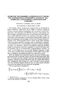
Table 2: Parameters of evolution. Symbolic regression Boolean domain Classifier induction Number of runs 30 Population size 1000 Fitness function L2 metric L1 metric Classification error Termination condition At most 50 generations or find of a program with fitness 0 Instructions x1 , x2 , +, −, ×, /, x1 , x2 , ..., x11 ,b x1 , x2 , ..., x9 , c1 , c2 , if sin, cos, exp, loga and, or, nand, nor a b

log is defined as log |x|; / returns 0 if divisor is 0. The number of inputs depends on a particular problem instance

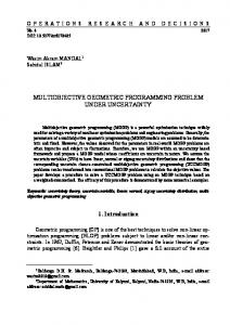
Table 3: Average and 95% confidence interval of fitness of the best of run program on training set. (a) Training-set fitness Problem R1 R2 R3 Kj1 Kj4 Ng9 Ng12 Pg1 Vl1 Par5 Par6 Par7 Mux6 Mux11 Maj7 Maj8 Cmp6 Cmp8 Cancer Rank:

LC GSGP 0.00 ±0.00 2.71 ±0.27 0.00 ±0.00 0.50 ±0.06 0.00 ±0.00 0.19 ±0.02 0.00 ±0.00 0.35 ±0.01 0.00 ±0.00 0.96 ±0.03 0.00 ±0.00 0.65 ±0.04 0.00 ±0.00 0.37 ±0.02 0.00 ±0.00 1.25 ±0.08 0.00 ±0.00 1.03 ±0.02 0.00 ±0.00 0.00 ±0.00 0.00 ±0.00 0.00 ±0.00 0.00 ±0.00 0.13 ±0.12 0.00 ±0.00 1.13 ±0.37 0.00 ±0.00 132.33 ±11.25 0.00 ±0.00 0.00 ±0.00 0.00 ±0.00 0.00 ±0.00 0.00 ±0.00 0.00 ±0.00 0.00 ±0.00 0.00 ±0.00 0.00 ±0.00 0.05 ±0.01 1.16 1.84

(b) Test-set fitness Problem R1 R2 R3 Kj1 Kj4 Ng9 Ng12 Pg1 Vl1 Cancer Rank:

LC 0.00 ±0.00 0.00 ±0.00 0.00 ±0.00 0.00 ±0.00 1.15 ±0.00 0.26 ±0.00 0.11 ±0.00 15.60 ±0.00 3.63 ±0.00 0.51 ±0.00 1.30

GSGP 17.25 ±0.83 3.20 ±0.05 0.67 ±0.01 0.51 ±0.01 2.25 ±0.07 5.85 ±0.05 2.11 ±0.01 7.34 ±0.07 3.35 ±0.02 0.04 ±0.01 1.70

produced programs. LC is run once for each problem, since it is deterministic. Presented CPU times are obtained on Intel Core i7-950 CPU and 6GB DDR3 RAM running in x64 mode under control of Linux and Java 1.8. The times exclude calculation of statistics. 4.2

Results

Table 3a presents average and 95% confidence interval of the best of run fitness. Since LC is guaranteed to construct the optimal program, it achieves 0 fitness and 0 confidence interval in each problem. In turn, GSGP is able to find the optimum only in 6 out of 19 problems. Wilcoxon signed rank test results in p-value of 1.66 × 10−3 , thus LC is statistically better than GSGP. Table 3b shows average and 95% confidence interval of test-set fitness of the best of run program on training-set. In 4 out of 10 problems LC achieves 0 fitness and is better than GSGP in 7 out of 10 problems. Wilcoxon test results in pvalue of 0.13, thus at significance level α = 0.05, the difference of generalization abilities of LC and GSGP is insignificant. Table 4a compares numbers of nodes in programs produced by LC and GSGP. In all 19 problems LC produces programs smaller by 1 up to 14 orders of magnitude than GSGP. Wilcoxon test results in p-value of 3.82 × 10−6 , which only

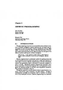
Table 4: Average and 95% confidence interval of: (a) number of nodes in the best of run program; values > 104 are rounded to an order of magnitude Problem R1 R2 R3 Kj1 Kj4 Ng9 Ng12 Pg1 Vl1 Par5 Par6 Par7 Mux6 Mux11 Maj7 Maj8 Cmp6 Cmp8 Cancer Rank:

LC GSGP 259.00 ±0.00 1016 ±1015 259.00 ±0.00 1015 ±1015 259.00 ±0.00 1016 ±1015 259.00 ±0.00 1015 ±1015 259.00 ±0.00 1015 ±1015 2099.00 ±0.00 1016 ±1015 2099.00 ±0.00 1015 ±1014 2099.00 ±0.00 1015 ±1014 1448.00 ±0.00 1015 ±1015 199.00 ±0.00 104 ±1327.87 479.00 ±0.00 106 ±105 1119.00 ±0.00 1015 ±1015 215.00 ±0.00 1016 ±1015 6776.00 ±0.00 1016 ±1015 1049.00 ±0.00 105 ±104 1719.00 ±0.00 105 ±6049.50 419.00 ±0.00 2467.60 ±350.10 2399.00 ±0.00 106 ±105 106 ±0.00 1016 ±1015 1.00 2.00

(b) total CPU time (seconds) Problem R1 R2 R3 Kj1 Kj4 Ng9 Ng12 Pg1 Vl1 Par5 Par6 Par7 Mux6 Mux11 Maj7 Maj8 Cmp6 Cmp8 Cancer Rank:

LC 0.03 ±0.00 0.03 ±0.00 0.03 ±0.00 0.02 ±0.00 0.03 ±0.00 0.08 ±0.00 0.08 ±0.00 0.09 ±0.00 0.08 ±0.00 0.04 ±0.00 0.06 ±0.00 0.06 ±0.00 0.05 ±0.00 0.79 ±0.00 0.08 ±0.00 0.13 ±0.00 0.05 ±0.00 0.07 ±0.00 0.19 ±0.00 1.00

GSGP 1.13 ±0.02 1.13 ±0.03 1.17 ±0.03 1.18 ±0.04 1.20 ±0.03 1.37 ±0.04 1.38 ±0.04 1.34 ±0.03 1.36 ±0.05 0.31 ±0.01 0.46 ±0.01 0.74 ±0.07 1.06 ±0.17 3.75 ±0.22 0.49 ±0.01 0.52 ±0.02 0.32 ±0.01 0.53 ±0.02 25.89 ±0.44 2.00

confirms our observation that LC produces smaller programs. Note that the numbers of nodes are equal in LC programs for all univariate, and all bivariate except Vl1 symbolic regression problems, respectively. This comes from the way how LC constructs the final program: basis for all problems with the same number of variables is exactly the same, only weights of the sum in Eq. (2) differ. LC program in Vl1 is smaller, because some of the weights in Eq. (2) are zero and the respective program parts are dropped. Last, but not least, Table 4b shows average and 95% confidence interval of CPU time required to finish the run. In each problem, LC run takes less than 0.8 second and is faster than the GSGP run. In contrast, GSGP requires 1 or 2 orders of magnitude more time, depending on a problem. Wilcoxon test reports p-value of 3.82 × 10−6 , hence LC is significantly faster than GSGP.

5

Discussion

GSGP builds overgrowth programs [18,27] that, due to its size, are difficult to interpret by humans, require a lot of a storage memory and possibly execute longer than smaller semantically equal programs. Since program simplification

is NP-hard in general [5], it is doubtful that any simplification procedure can reduce programs produced by GSGP (cf. Table 4a) to a human-interpretable size. Additionally, a program built by GSGP is a linear combination of the given program parts. This means that virtually any, random, unrelated conglomerates of instructions can be synthesized, and combined together using constant coefficients. The progress of evolution in GSGP is limited to adaptation of these coefficients, leaving the given program parts intact. This limits also the program’s ability to properly model a relation of input and output hidden in the training data, thus to properly operate on previously unseen data. The presented LC algorithm also constructs a program using a linear combination of arbitrarily synthesized program parts. This means that LC and GSGP share some of the drawbacks of this way of constructing programs, e.g., overfitting to the training data. Nevertheless, LC has advantages over GSGP. LC is twostep, deterministic and exact algorithm, i.e., it guarantees construction of the optimal program w.r.t. the given program induction problem in a polynomial time. On the other hand, GSGP iteratively and stochastically combines given programs, to gradually converge to the optimum, without a guarantee of reaching it or terminating. This difference makes the final programs constructed by LC smaller than by GSGP in all our experiments. LC is a naive approach that does not go beyond a toy example. In the field, there are many methods that construct either linear, or non-linear models that perform and generalize well in the considered class problems. For instance, in symbolic regression one can use Fast Function Extraction heuristic [14] or even assume a specific model and use one of classic regression or interpolation methods for it. In Boolean domain, the common approach is to use Karnaugh map minimization [8] that obviously produces smaller programs than LC. In classifier induction domain, one can use, e.g., decision trees or probabilistic classifiers [6]. This wide range of simple well performing methods, inclines us to claim that GSGP is overkill for problems of program induction stated as learning of function h : I → O. Where GSGP is useful? Though, it is important to say, that GSGP is not entirely doomed to fail. We can distinguish at least two features that makes GSGP useful in certain situations. First, consider target to be unknown and fitness function to be black-box that fulfils requirements of metric. All algorithms discussed in the previous section, except GSGP, require access to the target. This is because GSGP operators conduct strictly syntactic manipulations that have well-defined impact on program semantics, however the semantics itself is not used by the geometric operators. Second, GSGP can be split into broad theoretic framework with multiple achievements in the recent years [25,24,17,21,19,20,26] and algorithms of geometric operators. The main weakness of GSGP lies not in the former, but in the latter ones. GSGP theory does not define how to build offspring using parent programs, it only poses requirements to be met by the offspring (cf. Definitions 1 and 3). It is the algorithms are responsible for building linear combination of

random program parts, code growth and poor generalization. To the date, we do not have other algorithms than the presented in Definitions 2 and 4 that fulfil requirements of Definitions 1 and 3. However, there were multiple attempts to create approximate algorithms that on average or in the limit can fulfil these requirements, e.g., [10,11,28,23,24,22]. Nevertheless, future work is need in designing new exact algorithms for geometric operators that do not construct offspring by linearly combining parents.

6

Conclusions

Program induction problem in Geometric Semantic Genetic Programming is stated by means of learning function h : I → O. We demonstrated that GSGP in an attempt to solve this problem constructs a linear combination of random parts, however GSGP is not guaranteed to solve this problem optimally in finite time. We showed that the linear combination of random program parts can be constructed by much simpler means than GSGP with guarantee of solving the problem optimally. The optimal program is smaller than these of GSGP, and time consumed by the proposed algorithm is shorter and predetermined (polynomial). This, does not preclude practical use of GSGP, however a future work has to be done to put GSGP on the right track. We need new algorithms for GSGP operators that fulfil definitions of geometric operators (cf. Definitions 1 and 3), but do not operate by linearly combining parent programs in offspring.

Acknowledgements This work is funded by National Science Centre Poland grant number DEC-2012/07/N/ST6/03066.

References 1. R. Burden and J. Faires. Numerical Analysis. Cengage Learning, 2010. 2. M. Castelli, D. Castaldi, I. Giordani, S. Silva, L. Vanneschi, F. Archetti, and D. Maccagnola. An efficient implementation of geometric semantic genetic programming for anticoagulation level prediction in pharmacogenetics. In L. Correia, L. P. Reis, and J. Cascalho, editors, Proceedings of the 16th Portuguese Conference on Artificial Intelligence, EPIA 2013, volume 8154 of Lecture Notes in Computer Science, pages 78–89, Angra do Heroismo, Azores, Portugal, Sept. 9-12 2013. Springer. 3. M. Castelli, R. Henriques, and L. Vanneschi. A geometric semantic genetic programming system for the electoral redistricting problem. Neurocomputing, 154:200– 207, 2015. 4. M. Castelli, L. Vanneschi, and S. Silva. Prediction of high performance concrete strength using genetic programming with geometric semantic genetic operators. Expert Systems with Applications, 40(17):6856–6862, 2013.

5. N. Dershowitz and J.-P. Jouannaud. Rewrite systems. In Handbook of Theoretical Computer Science, Volume B: Formal Models and Sematics (B), pages 243–320. 1990. 6. P. Flach. Machine Learning: The Art and Science of Algorithms That Make Sense of Data. Cambridge University Press, New York, NY, USA, 2012. 7. J. E. Gentle. Numerical linear algebra for applications in statistics. Statistics and computing. Springer, New York, 1998. 8. M. Karnaugh. The map method for synthesis of combinational logic circuits. American Institute of Electrical Engineers, Part I: Communication and Electronics, Transactions of the, 72(5):593–599, Nov 1953. 9. J. R. Koza. Genetic Programming: On the Programming of Computers by Means of Natural Selection. MIT Press, Cambridge, MA, USA, 1992. 10. K. Krawiec and P. Lichocki. Approximating geometric crossover in semantic space. In G. Raidl, F. Rothlauf, G. Squillero, R. Drechsler, T. Stuetzle, M. Birattari, C. B. Congdon, M. Middendorf, C. Blum, C. Cotta, P. Bosman, J. Grahl, J. Knowles, D. Corne, H.-G. Beyer, K. Stanley, J. F. Miller, J. van Hemert, T. Lenaerts, M. Ebner, J. Bacardit, M. O’Neill, M. Di Penta, B. Doerr, T. Jansen, R. Poli, and E. Alba, editors, GECCO ’09: Proceedings of the 11th Annual conference on Genetic and evolutionary computation, pages 987–994, Montreal, 8-12 July 2009. ACM. 11. K. Krawiec and T. Pawlak. Locally geometric semantic crossover: a study on the roles of semantics and homology in recombination operators. Genetic Programming and Evolvable Machines, 14(1):31–63, Mar. 2013. 12. S. Luke. The ECJ Owner’s Manual – A User Manual for the ECJ Evolutionary Computation Library, zeroth edition, online version 0.2 edition, Oct. 2010. 13. O. L. Mangasarian, W. N. Street, and W. H. Wolberg. Breast cancer diagnosis and prognosis via linear programming. OPERATIONS RESEARCH, 43:570–577, 1995. 14. T. McConaghy. Ffx: Fast, scalable, deterministic symbolic regression technology. In R. Riolo, E. Vladislavleva, and J. H. Moore, editors, Genetic Programming Theory and Practice IX, Genetic and Evolutionary Computation, chapter 13, pages 235– 260. Springer, Ann Arbor, USA, 12-14 May 2011. 15. J. McDermott, A. Agapitos, A. Brabazon, and M. O’Neill. Geometric semantic genetic programming for financial data. In A. I. Esparcia-Alcazar and A. M. Mora, editors, 17th European Conference on the Applications of Evolutionary Computation, volume 8602 of LNCS, pages 215–226, Granada, 23-25 Apr. 2014. Springer. 16. J. McDermott, D. R. White, S. Luke, L. Manzoni, M. Castelli, L. Vanneschi, W. Jaskowski, K. Krawiec, R. Harper, K. De Jong, and U.-M. O’Reilly. Genetic programming needs better benchmarks. In T. Soule, A. Auger, J. Moore, D. Pelta, C. Solnon, M. Preuss, A. Dorin, Y.-S. Ong, C. Blum, D. L. Silva, F. Neumann, T. Yu, A. Ekart, W. Browne, T. Kovacs, M.-L. Wong, C. Pizzuti, J. Rowe, T. Friedrich, G. Squillero, N. Bredeche, S. L. Smith, A. Motsinger-Reif, J. Lozano, M. Pelikan, S. Meyer-Nienberg, C. Igel, G. Hornby, R. Doursat, S. Gustafson, G. Olague, S. Yoo, J. Clark, G. Ochoa, G. Pappa, F. Lobo, D. Tauritz, J. Branke, and K. Deb, editors, GECCO ’12: Proceedings of the fourteenth international conference on Genetic and evolutionary computation conference, pages 791–798, Philadelphia, Pennsylvania, USA, 7-11 July 2012. ACM. 17. A. Moraglio. Abstract convex evolutionary search. In H.-G. Beyer and W. B. Langdon, editors, Foundations of Genetic Algorithms, pages 151–162, Schwarzenberg, Austria, 5-9 Jan. 2011. ACM.

18. A. Moraglio, K. Krawiec, and C. G. Johnson. Geometric semantic genetic programming. In C. A. Coello Coello, V. Cutello, K. Deb, S. Forrest, G. Nicosia, and M. Pavone, editors, Parallel Problem Solving from Nature, PPSN XII (part 1), volume 7491 of Lecture Notes in Computer Science, pages 21–31, Taormina, Italy, Sept. 1-5 2012. Springer. 19. A. Moraglio and A. Mambrini. Runtime analysis of mutation-based geometric semantic genetic programming for basis functions regression. In C. Blum, E. Alba, A. Auger, J. Bacardit, J. Bongard, J. Branke, N. Bredeche, D. Brockhoff, F. Chicano, A. Dorin, R. Doursat, A. Ekart, T. Friedrich, M. Giacobini, M. Harman, H. Iba, C. Igel, T. Jansen, T. Kovacs, T. Kowaliw, M. Lopez-Ibanez, J. A. Lozano, G. Luque, J. McCall, A. Moraglio, A. Motsinger-Reif, F. Neumann, G. Ochoa, G. Olague, Y.-S. Ong, M. E. Palmer, G. L. Pappa, K. E. Parsopoulos, T. Schmickl, S. L. Smith, C. Solnon, T. Stuetzle, E.-G. Talbi, D. Tauritz, and L. Vanneschi, editors, GECCO ’13: Proceeding of the fifteenth annual conference on Genetic and evolutionary computation conference, pages 989–996, Amsterdam, The Netherlands, 6-10 July 2013. ACM. 20. A. Moraglio, A. Mambrini, and L. Manzoni. Runtime analysis of mutation-based geometric semantic genetic programming on boolean functions. In F. Neumann and K. De Jong, editors, Foundations of Genetic Algorithms, pages 119–132, Adelaide, Australia, 16-20 Jan. 2013. ACM. 21. A. Moraglio and D. Sudholt. Runtime analysis of convex evolutionary search. In T. Soule and J. H. Moore, editors, GECCO, pages 649–656. ACM, 2012. 22. Q. U. Nguyen, T. A. Pham, X. H. Nguyen, and J. McDermott. Subtree semantic geometric crossover for genetic programming. Genetic Programming and Evolvable Machines, 17(1):25–53, Mar. 2016. 23. T. Pawlak. Combining semantically-effective and geometric crossover operators for genetic programming. In T. Bartz-Beielstein, J. Branke, B. Filipic, and J. Smith, editors, 13th International Conference on Parallel Problem Solving from Nature, volume 8672 of Lecture Notes in Computer Science, pages 454–464, Ljubljana, Slovenia, 13-17 Sept. 2014. Springer. 24. T. P. Pawlak. Competent Algorithms for Geometric Semantic Genetic Programming. PhD thesis, Poznan University of Technology, Poznan, Poland, 21 Sept. 2015. 25. T. P. Pawlak and K. Krawiec. Guarantees of progress for geometric semantic genetic programming. In C. Johnson, K. Krawiec, A. Moraglio, and M. O’Neill, editors, Semantic Methods in Genetic Programming, Ljubljana, Slovenia, 13 Sept. 2014. Workshop at Parallel Problem Solving from Nature 2014 conference. 26. T. P. Pawlak and K. Krawiec. Progress properties and fitness bounds for geometric semantic search operators. Genetic Programming and Evolvable Machines, 17(1):5– 23, Mar. 2016. 27. T. P. Pawlak, B. Wieloch, and K. Krawiec. Review and comparative analysis of geometric semantic crossovers. Genetic Programming and Evolvable Machines, 16(3):351–386, Sept. 2015. 28. T. P. Pawlak, B. Wieloch, and K. Krawiec. Semantic backpropagation for designing search operators in genetic programming. IEEE Transactions on Evolutionary Computation, 19(3):326–340, June 2015. 29. C. Runge. Über empirische funktionen und die interpolation zwischen äquidistanten ordinaten. Zeitschrift für Mathematik und Physik, (46):224–243, 1901.

30. L. Vanneschi, S. Silva, M. Castelli, and L. Manzoni. Geometric semantic genetic programming for real life applications. In R. Riolo, J. H. Moore, and M. Kotanchek, editors, Genetic Programming Theory and Practice XI, Genetic and Evolutionary Computation, chapter 11, pages 191–209. Springer, Ann Arbor, USA, 9-11 May 2013. 31. Z. Zhu, A. K. Nandi, and M. W. Aslam. Adapted geometric semantic genetic programming for diabetes and breast cancer classification. In IEEE International Workshop on Machine Learning for Signal Processing (MLSP 2013), Sept. 2013.