University of Nebraska - Lincoln
DigitalCommons@University of Nebraska - Lincoln Biological Systems Engineering: Papers and Publications
Biological Systems Engineering
6-2010
Geophysical Mapping of Preferential Flow Paths across Multiple Floodplains Ronald B. Miller Oklahoma State University,
[email protected]
Derek M. Heeren University of Nebraska-Lincoln,
[email protected]
Garey A. Fox Oklahoma State University,
[email protected]
Daniel E. Storm Oklahoma State University,
[email protected]
Todd Halihan Oklahoma State University,
[email protected] See next page for additional authors
Follow this and additional works at: http://digitalcommons.unl.edu/biosysengfacpub Part of the Bioresource and Agricultural Engineering Commons, and the Civil and Environmental Engineering Commons Miller, Ronald B.; Heeren, Derek M.; Fox, Garey A.; Storm, Daniel E.; Halihan, Todd; and Mittelstet, Aaron R., "Geophysical Mapping of Preferential Flow Paths across Multiple Floodplains" (2010). Biological Systems Engineering: Papers and Publications. Paper 374. http://digitalcommons.unl.edu/biosysengfacpub/374
This Article is brought to you for free and open access by the Biological Systems Engineering at DigitalCommons@University of Nebraska - Lincoln. It has been accepted for inclusion in Biological Systems Engineering: Papers and Publications by an authorized administrator of DigitalCommons@University of Nebraska - Lincoln.
Authors
Ronald B. Miller, Derek M. Heeren, Garey A. Fox, Daniel E. Storm, Todd Halihan, and Aaron R. Mittelstet
This article is available at DigitalCommons@University of Nebraska - Lincoln: http://digitalcommons.unl.edu/biosysengfacpub/374
An ASABE Meeting Presentation Paper Number: 1008730
Geophysical Mapping of Preferential Flow Paths across Multiple Floodplains Ronald B. Miller, Ph.D. Student Oklahoma State University, Environmental Science, 111 Ag Hall, Stillwater, OK 74078,
[email protected]
Derek M. Heeren, Research Engineer and Ph.D. Student Oklahoma State University, Department of Biosystems and Ag Engineering, 114 Ag Hall, Stillwater, OK 74078,
[email protected]
Garey A. Fox, Ph.D., P.E., Associate Professor Oklahoma State University, Department of Biosystems and Ag Engineering, 120 Ag Hall, Stillwater, OK 74078,
[email protected]
Daniel E. Storm, Ph.D., Professor Oklahoma State University, Department of Biosystems and Ag Engineering, 121 Ag Hall, Stillwater, OK 74078,
[email protected].
Todd Halihan, Ph.D., Associate Professor Oklahoma State University, Boone Pickens School of Geology, 205 Noble Research Center, Stillwater, OK 74078,
[email protected]
Aaron R. Mittelstet, Research Engineer and Ph.D. Student Oklahoma State University, Department of Biosystems and Ag Engineering, 114 Ag Hall, Stillwater, OK 74078,
[email protected]
Written for presentation at the 2010 ASABE Annual International Meeting Sponsored by ASABE David L. Lawrence Convention Center Pittsburgh, Pennsylvania June 20 – June 23, 2010
The authors are solely responsible for the content of this technical presentation. The technical presentation does not necessarily reflect the official position of the American Society of Agricultural and Biological Engineers (ASABE), and its printing and distribution does not constitute an endorsement of views which may be expressed. Technical presentations are not subject to the formal peer review process by ASABE editorial committees; therefore, they are not to be presented as refereed publications. Citation of this work should state that it is from an ASABE meeting paper. EXAMPLE: Author's Last Name, Initials. 2010. Title of Presentation. ASABE Paper No. 10----. St. Joseph, Mich.: ASABE. For information about securing permission to reprint or reproduce a technical presentation, please contact ASABE at
[email protected] or 269-429-0300 (2950 Niles Road, St. Joseph, MI 49085-9659 USA).
Abstract. In the Ozark ecoregion of Oklahoma, Arkansas and Missouri, the erosion of carbonate bedrock (primarily limestone) by slightly acidic water has left a residuum of chert gravel, producing gravel-bed streams and floodplains generally consisting of coarse chert gravel overlain by a mantle (1 to 300 cm) of gravelly loam or silt loam. Previous research has documented the occurrence of preferential flow paths (PFP) in an alluvial floodplain hypothesized to be a buried gravel bar. Field experiments have shown that the PFP affected alluvial groundwater flow in the floodplain and that water flow in the PFP was transmitted at rates that limited sorption of phosphorus. The implication of these findings depends partly on the frequency and distribution of similar preferential flow features. To this end, four floodplain sites were chosen for comparative mapping. The sites were located in the Ozark region of northeast Oklahoma and had similar underlying geology but differed in watershed area, land cover, and stream order. Subsurface features at the sites were mapped using electrical resistivity imaging (ERI). Vadose zone hydraulic conductivity was measured at three sites using a direct-push borehole permeameter. The ERI profiles at each site showed that the subsurface was heterogeneous and areas of high electrical resistivity formed discrete, possibly continuous features in the vadose zone. Interpolations, based on variograms of resistivity, showed that resistivity within the alluvial aquifers formed patterns that were often linked to geomorphic processes. Hydraulic conductivity within the alluvial aquifers was estimated by applying an empirical linear relationship between electrical resistivity and hydraulic conductivity. Since all of the alluvial floodplain sites were gravel dominated systems, the sites were similar enough that the linear relationship between electrical resistivity and hydraulic conductivity was not site-specific. The positive slope of the relationship suggested that areas of continuous high resistivity could also act as zones of preferential flow within the aquifer under suitable hydrologic conditions. Among the sites, maximum electrical resistivity and hydraulic conductivity generally increased with increasing watershed area. Keywords. Electrical Resistivity, Hydraulic Conductivity, Preferential Flow, Subsurface Imaging
The authors are solely responsible for the content of this technical presentation. The technical presentation does not necessarily reflect the official position of the American Society of Agricultural and Biological Engineers (ASABE), and its printing and distribution does not constitute an endorsement of views which may be expressed. Technical presentations are not subject to the formal peer review process by ASABE editorial committees; therefore, they are not to be presented as refereed publications. Citation of this work should state that it is from an ASABE meeting paper. EXAMPLE: Author's Last Name, Initials. 2010. Title of Presentation. ASABE Paper No. 10----. St. Joseph, Mich.: ASABE. For information about securing permission to reprint or reproduce a technical presentation, please contact ASABE at
[email protected] or 269-429-0300 (2950 Niles Road, St. Joseph, MI 49085-9659 USA).
Introduction The chert-bearing carbonate geology of the Ozarks produces complex hydrologic flow patterns influenced by caves, sinkholes, springs, and also streams with beds and banks dominated by coarse chert gravel (Jacobson and Gran, 1999). However, in some parts of the Ozarks, stream and reservoir water quality is threatened, partly as a result of changes in land use that have increased nutrient concentrations and loads (Menjoulet et al., 2009). Alluvial floodplains are complex and dynamic landforms resulting from channel migration, fluvial erosion and sediment deposition, producing both vertical and horizontal spatial heterogeneity (Bridge, 2003). Previous work has documented complex subsurface flow patterns for graveldominated floodplains in the Ozarks. Using an array of monitoring wells designed to capture subsurface flow from an injection trench to a nearby stream, Fuchs et al. (2009) found a preferential flow path (PFP) that transported water bearing a conservative tracer (Rhodamine WT) and phosphorus (P) in a discrete direction in subsurface alluvial gravels. The tracer concentration found in the wells within the PFP (2 to 3 m from the trench) was similar to the concentration in the trench, while non-PFP wells located a similar distance from the trench had greatly reduced concentrations. The rate of transport in the PFP was found to overwhelm the potential for P sorption, allowing P to travel from the injection trench and along the PFP in relatively undiminished concentrations (Fuchs et al., 2009). Larger-scale transport experiments have also demonstrated the influence of the PFP, acting in accordance with the larger groundwater system dynamics, on conservative tracer transport (Heeren et al., 2010a, b). Subsurface PFPs are undetectable by visual inspection of the surface and thus mapping PFPs requires an indirect method. Electrical resistivity imaging (ERI) has been used to measure twoand three-dimensional profiles below the surface in near-surface applications. Auton (1992) and Beresnev et al. (2002) have used ERI for gravel prospecting, Gourry et al. (2003) and Green et al. (2005) for mapping buried paleochannels, and Smith and Sjogren (2006) for geologic investigation of glacial deposits. Baines et al. (2002) and Bersezio et al. (2007) are among those who have used ERI to map floodplain fluvial sediments, while Crook et al. (2008) used ERI to map the sedimentary structure of the active streambed itself. Researchers have noted that both Darcy’s Law of flow in porous media and Archie’s Law of resistivity (Archie, 1942) depend on the porosity of the matrix material, and theorized a relationship between the electrical resistivity of a porous media and its water transmitting characteristics (Lesmes and Friedman, 2005). Since the hydraulic properties of aquifers are difficult to accurately measure across large areas and ERI offers a relatively rapid and inexpensive window into the subsurface, this relationship has been sought as a way to estimate the hydraulic conductivity of aquifers. However, the relationship is not straightforward. Mazac et al. (1985) noted that previous work showed both positive and negative correlations between resistivity and hydraulic conductivity. Similarly, Dam et al. (2000) notes that while a general relationship between electrical resistivity and hydraulic conductivity has not been found, sitespecific empirical relationships can be effectively determined. Evaluating the importance of subsurface PFPs for planning and environmental modeling requires understanding their material nature and spatial distribution at the field and watershed scales. The objectives of this research were two-fold: (1) to assess the presence of potential high hydraulic conductivity PFPs in several alluvial floodplains sites, and (2) derive threedimensional hydraulic conductivity maps to better aid in understanding the movement of water and potential contaminants within the alluvial aquifers.
2
Materials and Methods Floodplain Field Sites The Ozark ecoregion of Missouri, Arkansas, and Oklahoma (Figure 1) is characterized by karst topography, including caves, springs, sink holes, and losing streams. The erosion of carbonate bedrock (primarily limestone) by slightly acidic water has left a large residuum of chert gravel in Ozark soils, with floodplains generally consisting of coarse chert gravel overlain by a mantle of gravelly loam or silt loam that ranges in thickness from 0.1 to 3 m. Topsoil depth in the floodplain generally increased with increasing stream order. Common soil series in the region include Elsah (frequently flooded, 0 to 3% slopes) in floodplains; Healing (occasionally flooded, 0 to 1% slopes) and Razort (occasionally flooded, 0 to 3% slopes) in floodplains and low stream terraces; Britwater (0 to 8 % slopes) on high stream terraces; and Clarksville (1 to 50%) on bluffs. Four sites were selected on a variety of streams within the Ozark region of northeastern Oklahoma (Figure 1). Watershed size and land use varied at each site (Table 1).
Figure 1. Location of the selected floodplain sites in northeastern Oklahoma.
3
Table 1. Land use and watershed characteristics of the studied floodplain sites. Watershed Area (km2)
Median Daily Discharge1 (m3 s-1)
Primary Land Use
Barren Fork Creek
845
3.6
Hay field
Flint Creek
300
1.6
Riparian forest, hay field
Honey Creek
150
0.54
Riparian forest, hay field
Pumpkin Hollow
15
Intermittent
Pasture
Site
1
Source: U.S. Geological Survey
Electrical Resistivity Imaging Electrical Resistivity Imaging (ERI) is a geophysical method commonly used for near-surface investigations which measures the resistance of earth materials to the flow of DC current between two source electrodes. The method is popular because it is efficient and relatively unaffected by many environmental factors that confound other geophysical methods. According to Archie’s Law (Archie, 1942), earth materials offer differing resistance to current depending on grain size, surface electrical properties, pore saturation, and the ionic content of pore fluids. Normalizing the measured resistance by the area of the subsurface through which the current passes and the distance between the source electrodes produces resistivity, reported in ohmmeters ( Ω-m), is a property of the subsurface material (McNeill, 1980). Mathematical inversion of the measured voltages produces a two-dimensional profile of the subsurface showing areas of differing resistivity (Loke and Dahlin, 2002, Halihan et al., 2005). ERI data were collected using a SuperSting R8/IP Earth Resistivity Meter (Advanced GeoSciences Inc., Austin, TX) with a 56-electrode array. The ERI surveys at the four sites occurred between June 2008 and March 2009. Fourteen lines were collected at the Barren Fork Creek site, five at the Honey Creek site, four at the Flint Creek site, and three at the Pumpkin Hollow site. One line at the Barren Fork Creek site and all of the lines at Flint Creek and Pumpkin Hollow were “roll-along” lines that consisted of sequential ERI images with one-quarter overlap of electrodes. The profiles at the Barren Fork Creek site employed electrode spacing of 0.5, 1.0, 1.5, 2.0 and 2.5 m with associated depths of investigation of approximately 7.5, 15.0, 17.0, 22.5 and 25.0 m, respectively. All other sites utilized a 1-m spacing. The area of interest in each study site was less than 3 m below the ground surface and thus well within the ERI window. The resistivity sampling and subsequent inversion utilized a proprietary routine devised by Halihan et al. (2005), which produced higher resolution images than conventional techniques. The OhmMapper (Geometrics, San Jose, CA), a capacitively-coupled dipole-dipole array, was effectively deployed at the relatively open Barren Fork Creek site for large scale mapping. The system used a 40 m array (five 5 m transmitter dipoles and one 5 m receiver dipole with a 10 m separation) that was pulled behind an ATV. Two data readings per second were collected to create long and data-dense vertical profiles. The depth of investigation was limited to 3 to 5 m. Positioning data for the ERI and OhmMapper were collected with a TopCon HyperLite Plus GPS with base station. Points were accurate to within 1 cm.
4
Three-Dimensional Interpolation The ERI profiles were collected to assess the heterogeneity within the subsurface of the alluvial floodplains. The profiles themselves were two-dimensional and provided insight into only a small proportion of the subsurface. Interpolation between the ERI lines can provide insight into the possible distribution of resistivity across the entire floodplain study area. Variograms are a representation of spatial variation created by measuring the sum of squared differences of data pairs separated by every possible distance within the data set (Isaaks and Srivastava, 1989). The variogram components included the “nugget” or latent error of the estimate and the “range or the maximum distance for covariance between data points”. The variogram also included the angle and shape of anisotropy, which provided insight into the directionality of the closest relationship within the data. This was important in the context of PFPs since the angle of anisotropy could correspond to the flow direction within connected PFPs. A mathematical model (i.e., linear, quadratic, polynomial, exponential, etc.) fit to the variogram used the spatial variation within the data to interpolate values for the unsampled area. The variograms were generated using Surfer 8 (Golden Software, Golden, CO). Each site was modeled by selecting ERI data from a single elevation or horizontal “slices”. Slices were generated from the vadose zone of each site by estimating the baseflow water table elevation and then fitting as many slices as possible at 1 m increments. Several variograms were generated for each slice and used to interpolate the elevation “slice”. The resulting grid with the lowest standard deviation of variance was selected.
Saturated Hydraulic Conductivity At three of the field sites (Barren Fork Creek, Honey Creek, and Flint Creek), Miller et al. (2010) measured hydraulic conductivity (K) using a modification of existing borehole permeameter techniques. The alluvial gravels encountered at the study sites required a cased hole to prevent collapse and powerful drilling techniques to reach the intended depths. To circumvent this shortfall, a slotted casing was devised that could be driven to a specific depth. The screen section consisted of an 8.25-cm pipe section with 27 vertical slots (0.002 m wide by 0.2 m long) arranged in three groups with solid (unslotted) sections in between. This arrangement was chosen to provide the pipe strength to resist the forces necessary to penetrate the coarse gravels at each site. The screened area was 0.01 m2 with a ratio of open area to total area of 21%. The screen section allowed hydraulic conductivity testing of discrete depths of the floodplain vadose zone. A Geoprobe Systems (Salina, KS) 6200 TMP (trailer-mounted probe) direct-push drill rig was used to push the array of 8.25-cm diameter pipe sections to specified depths in the alluvial floodplain at each site. The K testing consisted of driving the screened section to the desired depth, installing a vented pressure transducer at the bottom of the well, placing a water inflow pipe on the open end of the pipe, and pumping water into the well from a 3.8 m3 portable tank. Testing in the well was initiated after the well reached a constant head (pseudo steady-state), usually after 10 to 15 minutes, and monitored with a pressure transducer. When necessary, flow into the well was adjusted with an in-line gate valve. Tests lasted approximately 15 minutes after reaching steady state, during which head in the well and level in the tank were recorded continuously. The flow into the well (Q, m3 s-1) was calculated using a stage/volume relationship for the tank and the total elapsed time for the test. The Q and stage data were converted to hydraulic conductivity using the U. S. Bureau of Reclamation Gravity Permeability Method 2 test for permeability of unsaturated material (USBR, 1985). Each test produced a value of field saturated hydraulic conductivity, Kfs, which can be less than saturated hydraulic conductivity (K), especially in fine-grained soils with high capillarity. The
5
gravel-dominated strata tested in this study had low capillarity and thus the measured Kfs was assumed to approximate the actual K. The test was valid for test conditions where the saturated thickness (S), was less than 5l, where l is the length of the screen section; l greater than or equal to 10r1, where r1 is the outside radius of the casing; and Q/a less than or equal to 0.10, where a was the perforated area of the screen. Some tests, especially those with the highest Q into the permeameter, failed these requirements and were removed from further analysis. Approximately 20 measurements of K from the three field sites satisfied the abovementioned criteria. The K value was assumed to occur at the depth of the screen for each test. Depth and the test position on the ERI line were used to determine the resistivity from the formation that was influencing the K measurement. The electrical resistivity value was determined by averaging the four inverted resistivity values closest to that point. An empirical relationship was derived between K and electrical resistivity similar to Miller et al. (2010). Distributions of K within the three alluvial aquifers were estimated by transforming resistivity values from the threedimensional ERI interpolations.
Results and Discussion Electrical Resistivity Imaging Results The ERI profiles showed heterogeneity of resistivity at each site as evidenced by the strong positive skew of resistivity values and the large number of extreme values seen in the resistivity boxplots (Table 2, Figure 2). The Barren Fork Creek site contained the most extreme resistivity range and the highest mean and maximum values, while the Honey Creek site had the highest median value.
Table 2. Descriptive statistics for vadose zone resistivity at the four study sites. All values are electrical resistivity in Ω-m. Standard Mean Deviation
Minimum
Median
Maximum
Barren Fork Creek
534
829
10.9
276
19100
Flint Creek
239
185
32.8
187
2500
Honey Creek
351
228
3.0
313
2430
Pumpkin Hollow
387
351
57.7
263
3110
6
Figure 2. Boxplot of vadose zone resistivity at each site. BF = Barren Fork Creek, FLCR = Flint Creek, HCr = Honey Creek, and PuHo = Pumpkin Hollow. The ERI profiles suggested that the resistivity was distributed heterogeneously with discrete areas of high and low resistivity (Figure 3). An increase in resistivity with depth was observed at all sites with the highest resistivities (> 5000 Ω-m) occurring at least 5 m below ground surface. These high values were consistent with the range of resistivity for limestone (1 x 10³ to 1 x 10⁷ Ω-m), and was interpreted as competent bedrock. Lower resistivity layers above the bedrock corresponded to gravel or weathered limestone (i.e., epikarst). Indirect evidence for this interpretation comes from the Honey Creek site where push-probe installation of monitoring wells encountered refusal at depths above the zone interpreted as bedrock (Heeren et al., 2010a). Among the sites, maximum electrical resistivity generally increased with increasing watershed area (Table 2). It is hypothesized that larger order streams would have sediment transport capacities capable of moving larger particle sizes, producing higher resistivities in stream deposited gravel. However, the relationship between stream or watershed characteristics and resistivity was not always consistent, since the factors influencing fluvial geomorphology varied among the sites. For example, Pumpkin Hollow had the smallest area but the second highest mean and maximum resistivity. This was likely due to gravel transported onto the floodplain from nearby plateau surfaces, with the hillslopes able to transport larger gravel than the stream. Site-specific characteristics were also important at the Flint Creek site. While both the Barren Fork Creek and Honey Creek sites were dominated by their resident streams, the Flint Creek floodplain may have been primarily constructed by a smaller, seasonal tributary (6.2 km2 watershed area), resulting in a low mean resistivity compared to Flint Creek’s watershed area (300 km2).
7
Figure 3. Example resistivity profiles from each site. All sites show horizontal distribution of high resistivity lenses in the vadose zone near the soil surface. Shallow depth to bedrock is evident in Honey Creek and Pumpkin Hollow profiles but the depth of investigation is too shallow to capture bedrock at the Flint Creek and Barren Fork Creek sites. The horizontal layer of lowresistivity at Pumpkin Hollow is interpreted as soil layer buried by gravel from nearby slopes. The y-axes are elevation above mean sea level (m) and the x-axes are lateral distance (m).
8
The depth of most interest for this project was the vadose zone or the area above the baseflow water table. This was the zone that controlled interaction between the ground surface and alluvial groundwater. Heterogeneity of resistivity within this zone was of particular interest because it could indicate the presence of PFPs. The sites, except Pumpkin Hollow, possessed a pattern of discrete high resistivity features within this zone, although the size and range of resistivities for these features varied. A detailed description of resistivity patterns within the zone of interest for each site follows. Field experience at the sites allows resistivities less than 100 Ω-m to be generally interpreted as fine-grained soils, 100 to 250 Ω-m as soil with gravel, 250 to 1000 Ω-m as gravel with fines, and >1000 Ω-m as clean gravel.
Barren Fork Creek Resistivity at the Barren Fork Creek site appeared to conform generally to surface topography with higher elevations having higher resistivity, although the net relief was minor (~1 m). This was most evident in the OhmMapper resistivity profiles which covered most of the floodplain and which revealed a pattern of high and low resistivity that trended SW to NE (Figure 4). More precise imaging with reduced spatial coverage was obtained with the ERI. The area around the PFP was clearly imaged with the roll-along and cross lines 1 to 5 (0.5 to 1 m electrode spacing), as shown in Figure 5. This feature appeared be 1 to 2 m thick, trended SW to NE (similar to the pattern seen in the OhmMapper survey), dipped slightly down to the SW, and ranged in width from 3 to 5 m. Other high resistivity features seen in the OhmMapper survey were detected by the longer ERI lines; for example, a relatively high resistivity feature was observed at 30 m on line 11, 70 m on line 13, 80 m on line 12, and then again at 70 m on lines 7 and 8 (Figure 5). This feature formed an angle of about 50° from an EW line, but because of the wider electrode spacing, those profiles had less resolution so the dimensions of the feature were not as clear (Figure 5).
Figure 4. OhmMapper coverage of the Barren Fork Creek alluvial floodplain showing SW to NE trends of low (blue) and high (orange) resistivity. View is to the North and subsurface resistivity profiles are displayed above the aerial image for visualization purposes. Modified from Heeren et al. (2010b).
9
Figure 5. High resistivity feature locations on ERI lines at the Barren Fork Creek site (shown in blue). The orientation of the arrow representing potential connections in high resistivity was similar to high resistivity features seen in OhmMapper profiles (Figure 4).
The linear nature and NE-SW directional trend of these surface features, roughly parallel to the stream, suggested that they might be old stream channels and lateral gravel bars buried by floodplain sediment. Evidence that some of the high resistivity features within these floodplains were likely to be gravel bars was derived from ERI evidence where an ERI profile from an exposed mid-channel gravel bar at this site suggested resistivities in the same range as those in the PFP area (1000 to 5000 Ω-m). Also, gravel material collected from the surface of the bar was similar in particle-size distribution to material from the stream bank at the PFP, with the percent of soil less than 2.0 mm diameter in the PFP and the gravel bar approximately 6% and 13% by mass, respectively (Heeren et al., 2010b). This comparison became available due to severe stream bank migration which revealed a section of the PFP.
Honey Creek The baseflow water table at the Honey Creek site was at an elevation of approximately 234 m. The ground surface elevation was between 235 and 236 m. Four ERI profiles (1 m electrode spacing and 12.5 m profile depth) were collected with a general S-N orientation. Resistivity
10
within the zone of interest ranged from less than 10 to 2400 Ω-m, with a mean of 351 Ω-m. Similar to the Barren Fork Creek site, it was observed that areas of high resistivity within the zone of interest at Honey Creek appeared in discrete units 2 to 5 m wide and about 1 m thick and were associated with high topographic features. However, the ERI profiles were not spaced close enough to conclusively determine connectivity between the high resistivity features (Figure 6). Considering that the site was located on the inside of a meander bend, an area considered to be an aggradational point bar (Bridge, 2003), the high resistivity features may be sequential deposits that retain the curvilinear shape of the meander bend (Figure 6). The stream was presently depositing coarse gravel on the point bar and thus it was reasonable to assume that historic deposits contained gravel as well.
Figure 6. High resistivity feature locations on ERI lines at the Honey Creek site (shown in blue). The curved line represents the potential connection in high resistivity.
Flint Creek The Flint Creek site occupied a narrow floodplain currently being eroded. Five separate ERI profiles, including three composite roll-along lines were collected. Each line was oriented orthogonal to the creek and as close to W-E as possible considering the riparian forest cover. Each profile had a 1 m electrode spacing and 12.5 m depth of investigation. The general alluvial floodplain surface elevation was about 267 m and the water table elevation about 265 m, so the area of interest extended approximately 2 m in depth. The range of resistivity found in
11
the ERI profiles within the alluvial interest area was 33 to 2500 Ω-m, with a mean of 239 Ω-m, and a distribution similar to the Honey Creek site (Figure 2). The vertical distribution of resistivity at the Flint Creek site was unique among sites studied because the profiles showed considerable variation in resistivity with depth. For instance, line 1 resulted in high resistivity close to the surface, which was likely to be a bedrock similar to an outcrop directly across the stream, while roll-along lines 2-3, 5-6 and 4-7 all showed a marked decrease in resistivity at the bottom of the profile suggesting that the bedrock seen in line 1 had dipped strongly to the north (Figure 7). Except line 1, the profiles had discrete areas of high resistivity ranging from 10 m in width in the northern lines to 1 m in lines 2-3. The high resistivity was likely due to gravel lenses within the floodplain, although the source may not be Flint Creek itself but rather a tributary that crosses the floodplain in the vicinity of line 8 (Figure 7).
Figure 7. High resistivity feature locations on ERI lines at the Flint Creek site (shown in blue). The line with an arrow represents potential high resistivity connection and the direction of flow.
12
Pumpkin Hollow Pumpkin Hollow differed from the other streams because it was a headwater stream with a smaller watershed area. The valley at the study site was approximately 200 m wide and the roll-along lines spanned nearly the entire valley width, crossing Pumpkin Hollow Creek at about the midpoint of the line. The ERI survey at Pumpkin Hollow consisted of three lines oriented WE with 1 m electrode spacing, 12.5 m depth, and 97 m (lines 1-2 and 3-4) or 139 m (line 5-6-7) length (Figure 8).
Figure 8. High resistivity feature locations on ERI lines at the Pumpkin Hollow site are shown in blue. Arrows represent potential connections between them and the direction of flow. The Pumpkin Hollow ERI profiles also had a unique configuration consisting of a low resistivity layer between a high resistivity surface layer and high resistivity at depth (Figure 3). The surface layer was dominated by gravel underlying only 1 to 3 cm of topsoil. Observations at the site included the close proximity of large gravel debris fans originating from nearby upland areas. Jacobson and Gran (1999) noted similar pulses of gravel in Ozark streams in Missouri and Arkansas originating from 19th and early 20th century deforestation of plateau surfaces,
13
implying that a possible interpretation of the low resistivity layer in the ERI profiles was a soil layer buried by gravel from the nearby plateau surfaces. The streambed elevation was approximately 262 m with the general floodplain surface being about 1 m above that elevation. Pumpkin Hollow was not actively flowing through the study site although flow was evident within 1 km downstream, suggesting that significant amounts of water were likely flowing within the gravel streambed as groundwater. The area of interest included the elevations above 262 m (note that the mean elevation was 262.9 m and that the maximum elevation 265 m occurred at the valley edge) and was therefore thin compared to the other study sites. The resistivity at Pumpkin Hollow ranged from 58 to 3110 Ω-m with a mean of 387 Ω-m. The mean and maximum values were ranked second behind only Barren Fork Creek and were additional evidence that the floodplain was dominated by gravel. Like the other sites, the Pumpkin Hollow resistivity suggested a pattern of discrete areas of high resistance that indicated PFPs (Figure 8). These were generally associated with topographic high areas and appeared to have the potential to direct flow down-valley parallel to the stream.
Three-Dimensional Interpolation The variograms generated for each site showed both variations among sites but also occasional variation between elevations within a site (Table 3). The anisotropy angle for variograms at the Barren Fork Creek was consistent with depth and generally corresponded to the PFP pattern detected on the ERI profiles. The anisotropy angles for the Pumpkin Hollow interpolations also were fairly consistent with depth and were also similar to the angle determined from the ERI profiles. The variograms at the Flint Creek and the Honey Creek sites both showed different angles with depth. The variety of anisotropy angles for the Flint Creek and the Honey Creek sites were possibly due to the presence of many similar features which can be linked at different angles indicating the presence of layers with different geomorphic origins. Table 3. Variogram model information for each of the selected alluvial floodplain sites. Elevation (m)
Barren Fork Creek Honey Creek Flint Creek Pumpkin Hollow
Standard Deviation
Nugget Effect
Model
Anisotropy Angle (degrees)
Range (m)
209
2060
6.88E+06
Power
46
1
210
564
1.19E+06
Power
50
1
211
213
1.63E+05
Power
50
2
234
99
4.97E+04
Power
44
1
235
111
2.50E+04
Linear
139
2
265
90
8.70E+03
Exponential
65
10
266
85
3.14E+03
Power
130
30
262
66
2.00E+00
Exponential
85
17
263
353
6.20E+03
Quadratic
97
78
14
Three elevation “slices” at the Barren Fork Creek were spaced at 1 m depth intervals designed to include the area between the baseflow water table (209 m) and the soil layer (211 m). The Barren Fork Creek surface interpolations show the high resistivity near the PFP and the low and high pattern that corresponded to surface topography (Figure 9). The resistivity consistently increased with depth so that high resistivity was typically continuous just above the water table.
3974750
211 meters
3974700
3974650
3974750
210 meters
3974700
3974650
3974750
209 meters
3974700
3974650 332600
332650
332700
332750
Ohm-m 2000
1000
500
350
275
200
150
100
20
5
Figure 9. Interpolated ERI surfaces for elevation slices at the Barren Fork Creek site. North is top of image. The Barren Fork Creek flows southwest along the top left edge. The interpolated surfaces are trimmed to the existing field of monitoring wells at the study site. Axes (m) are Eastings and Northings (UTM Zone 15N).
15
The Honey Creek site interpolations showed only a slight pattern of increase with depth with the highest connectivity among high resistivity occurring at higher elevations within the floodplain (Figure 10). The interpolated resistivity did not follow the curvilinear pattern that would be likely within point bar sediments, but that result could be explained due to the large area with little data at the apex of the curve, and because the variogram-based interpolation connected the existing points linearly.
235 meters
4045280 4045270 4045260 4045250 4045240 4045230
347410
347430
347450
347470
347490
234 meters
4045280 4045270 4045260 4045250 4045240 4045230
347410
347430
347450
347470
347490
Ohm-m 2000
1000
500
350
275
200
150
100
20
5
Figure 10. Interpolated ERI surfaces for elevation slices at the Honey Creek site. North is at the top of the image. Honey Creek flows westerly about 50 m south along the arc at the bottom. Axes (m) are Eastings and Northings (UTM Zone 15N).
16
The Flint Creek interpolation showed that resistivity increased with depth (Figure 11). The interpolations also showed a change in patterns: at the shallower depth there was a strong pattern across the alluvial floodplain to the stream while the deeper interpolation showed the longitudinal pattern parallel to the stream seen on the ERI profiles.
4007400
265 meters
4007400
4007380
4007380
4007360
4007360
266 meters
Ohm-m 2000
4007340
1000
4007340
500
4007320
350
4007320
275 200
4007300
4007300 150 100
4007280
4007280
20 5
4007260
4007260 346400
346420
346440
346460
346400
346420
346440
346460
Figure 11. Interpolated ERI surfaces for elevation slices at the Flint Creek site. North is at top of image. Flint Creek flows south on the east edge of site. Axes (m) are Eastings and Northings (UTM Zone 15N).
The Pumpkin Hollow interpolations showed a decrease in resistivity with depth that was most likely associated with the feature previously interpreted as a buried soil surface (Figure 12). The high resistivity in the shallower interpolation showed a longitudinal pattern parallel to the stream similar to that seen in the ERI profiles.
17
3987000
262 meters
3987000
3986980
3986980
3986960
3986960
3986940
3986940
3986920
3986920
3986900
3986900
3986880
3986880
3986860
3986860 336860
336880
336900
336920
336960
336860
336880
336900
336920
336940
336960
2000
1000
500
350
275
200
150
100
20
5
Ohm-m
336940
263 meters
Figure 12. Interpolated ERI surfaces for elevation slices at the Pumpkin Hollow site. North is at top of image. Pumpkin Hollow flows south through the center of the site. Axes (m) are Eastings and Northings (UTM Zone 15N).
Saturated Hydraulic Conductivity The goal of the ERI imaging was to produce a physically-based estimate of the spatial distribution of hydraulic conductivity (K) within the alluvial aquifers included in the study. Threedimensional grids of K were required for the understanding of flow within the alluvial system. To that end, an empirical, linear relationship between electrical resistivity, ρ (Ω-m), and K (m d-1) was established using borehole permeameter tests at the Barren Fork Creek, Honey Creek and Flint Creek study sites (Figure 13):
K = 0.105ρ
(1)
The regression had a coefficient of determination (R2) of 0.73 and the F-statistic was significant at α = 0.05. Since all of the alluvial floodplain sites were gravel dominated systems, the sites were similar enough in geology that the linear relationship between electrical resistivity and hydraulic conductivity was not site-specific. The interpolated ERI surfaces were based on a 2-m by 2-m grid of resistivity values and then converted to K using equation (1). The patterns revealed in the ERI interpolations were retained in K surfaces because the equation was a linear transformation. The positive slope of the relationship implied that areas with high resistivity also have high K, and that continuous high resistivity features may act as PFPs when hydrologic conditions are appropriate (during periods of high stream flow or surface runoff). Since maximum electrical resistivity generally increased with increasing watershed area, maximum hydraulic conductivity also generally increased with increasing watershed area
18
among the alluvial floodplain sites (Table 4). The maximum K at the Barren Fork Creek site (1752 m/d) was within the range for gravel reported by Domenico and Schwartz (1990).
Figure 13. Electrical resistivity versus saturated hydraulic conductivity measured with modified borehole permeameter tests (Miller et al., 2010) at the Barren Fork Creek, Flint Creek, and Honey Creek field sites.
Table 4: Summary statistics for interpolated hydraulic conductivity (K, m/d) at each site.
Barren Fork Flint Creek Honey Creek Pumpkin Hollow
Mean
Standard Deviation
Minimum
Median
Maximum
45 28 40 29
72 11 11 16
8 9 16 8
27 26 39 25
1750 98 80 176
Conclusions The ERI profiles showed that the subsurface was heterogeneous at each site and areas of high electrical resistivity formed discrete, possibly continuous features in the vadose zone. Interpolations, based on variograms of resistivity, showed that resistivity within the alluvial
19
aquifers formed patterns that were often linked to geomorphic processes. Saturated hydraulic conductivity within the alluvial aquifers was estimated by applying an empirical relationship between electrical resistivity and hydraulic conductivity. The linear relationship between electrical resistivity and hydraulic conductivity was not site-specific. The positive slope of the relationship suggested that areas of continuous high resistivity may act as zones of preferential flow within the aquifer under suitable hydrologic conditions. Among the sites, maximum electrical resistivity and hydraulic conductivity generally increased with increasing watershed area.
Acknowledgements This material was based upon work supported by the Oklahoma Conservation Commission with a U.S. Environmental Protection Agency Region VI 319 grant. The authors acknowledge Sharon Beck, Bill Berry, Dan Butler and Shannon Tate for providing access to their alluvial floodplain property. The authors also acknowledge Wayne Kiner and the Biosystems and Agricultural Engineering Laboratory staff, Oklahoma State University, for fabrication and essential machine maintenance, and Dr. Maria Chu-Agor, Jorge Guzman, and Tim Sickbert for assistance in the field.
References Archie, G.E. 1942. The electrical resistivity log as an aid in determining some reservoir characteristics. Petroleum Technology Technical Paper 1422. Auton, C.A. 1992. The utility of conductivity surveying and resistivity sounding in evaluating sand and gravel deposits and mapping drift sequences in northeast Scotland. Engineering Geology 32: 11-28. Baines, D., D.G. Smith, D.G. Froese, and P. Bauman. 2002. Electrical resistivity ground imaging (ERGI): A new tool for mapping the lithology and geometry of channel-belts and valleyfills. Sedimentology 49: 441-449. Beresnev, I.A., C.E. Hruby, and C.A. Davis. 2002. The use of multi-electrode resistivity imaging in gravel prospecting. Journal of Applied Geophysics 49: 245-254. Bersezio R., M. Giudici, and M. Mele. 2007. Combining sedimentological and geophysical data for high-resolution 3-D mapping of fluvial architectural elements in the Quaternary Po Plain (Italy). Sedimentary Geology 202(1-2): 230-248. Bridge, J.S. 2003. Rivers and Floodplains: Forms, Processes, and Sedimentary Record. Oxford, UK: Blackwell Publishing. Crook, N., A. Binley, R. Knight, D.A. Robinson, J. Zarnetske, and R. Haggerty. 2008. Electrical resistivity imaging of the architecture of substream sediments. Water Resources Research 44, W00D13, doi:10.1029/2008WR006968. Dam, D., S. Christensen, and N. B. Christensen. 2000. Characterizing the hydraulic conductivity field using electrical resistivity and inverse modeling. In Groundwater 2000: Proceedings of the International Conference on Groundwater Research, Copenhagen, Denmark, Bjerg P.L., P. Engesgaard, and T.D. Krom (eds). Balkema: Rotterdam, The Netherlands. Domenico, P.A., and F. W. Schwartz. 1990. Physical and Chemical Hydrogeology. New York, NY: John Wiley and Sons. Fuchs, J.W., G.A. Fox, D.E. Storm, C. Penn, and G.O. Brown. 2009. Subsurface transport of phosphorus in riparian floodplains: Influence of preferential flow paths. Journal of Environmental Quality 38(2): 473-484.
20
Gourry, J-C., F. Vermeersch, M. Garcin, and D. Girot. 2003. Contribution of geophysics to the study of alluvial deposits: a case study in the Val d’Avaray area of the River Loire, France. Journal of Applied Geosciences 54: 35-49. Green, R.T., R.V. Klar, and J.D. Prikryl. 2005. Use of integrated geophysics to characterize paleo-fluvial environments, Geotechnical Special Publication 138: Site Characterization and Modeling, ASCE, New York, NY. Halihan, T., S. Paxton, I. Graham, T. Fenstemaker, and M. Riley. 2005. Post-remediation evaluation of a LNAPL site using electrical resistivity imaging. Journal of Environmental Modeling 7: 283-287. Heeren, D.M., R.B. Miller, G.A. Fox, D.E. Storm, A.K. Fox, and A.R. Mittelstet. 2010a. Impact of preferential flow paths on stream and alluvial groundwater interaction. In Proc. ASCE EWRI World Environmental and Water Resources Congress. Reston, Va.: American Society of Civil Engineers. Heeren, D.M., R.B. Miller, G.A. Fox, D.E. Storm, C.J. Penn, and T. Halihan. 2010b. Preferential flow path effects on subsurface contaminant transport in alluvial floodplains. Transactions of the ASABE 53(1): 127-136. Isaaks E.H., and R.M. Srivastava. 1989. An Introduction to Applied Geostatistics. New York, N.Y.: Oxford University Press. Jacobson, R.B., and K.B. Gran 1999. Gravel sediment routing from widespread, low-intensity landscape disturbance, Current River Basin, Missouri. Earth Surface Processes and Landforms 24: 897-917. Lesmes, D.P, and S.P. Friedman. 2005. Relationship between the electrical and hydrogeological properties of rocks and soils. In Hydrogeophysics, Rubin, Y., and S.S. Hubbard (eds). Springer: Dordrecht, The Netherlands. Loke, M.H., and T. Dahlin. 2002. A comparison of the Gauss–Newton and quasi-Newton methods in resistivity imaging inversion. Journal of Applied Geophysics 49: 149–162. Mazac, O., W.E. Kelly, and I. Landa. 1985. A hydrological model for relations between electrical conductivity ad hydraulic properties of aquifers. Journal of Hydrology 79: 1-19. McNeill, J.D. 1980. Electrical Conductivity of Soils and Rocks. Technical Note TN-5, Geonics Limited, Ontario, Canada. Menjoulet, B.C., K.R. Brye, A.L. Pirani, B.E. Haggard, and E.E. Gbur. 2009. Runoff water quality from broiler-litter-amended tall fescue in response to natural precipitation in the Ozark Highlands. Journal of Environmental Quality 38: 1005-1017. Miller, R.B., D.M. Heeren, G.A. Fox, T. Halihan, D.E. Storm, and A.R. Mittelstet. 2010. Use of multi-electrode resistivity profiling to estimate vadose-zone hydraulic properties of preferential flow paths in alluvial floodplains. In Proc. ASCE EWRI World Environmental and Water Resources Congress. Reston, Va.: American Society of Civil Engineers. Smith, R.C., and D.B. Sjogren. 2006. An evaluation of electrical resistivity imaging (ERI) in Quaternary sediments, southern Alberta, Canada. Geosphere 2(6): 287-298. U.S. Bureau of Reclamation (USBR). 1985. Ground Water Manual: A Water Resources Technical Manual Revised Reprint. Denver, CO. U.S. Department of the Interior, Bureau of Reclamation.
21