GLOBAL VARIANCE EQUALIZATION FOR IMPROVING DEEP NEURAL NETWORK BASED SPEECH ENHANCEMENT Yong Xu† , Jun Du† , Li-Rong Dai† , and Chin-Hui Lee‡ †
National Engineering Laboratory for Speech and Language Information Processing, University of Science and Technology of China, P. R. China ‡ School of Electrical and Computer Engineering, Georgia Institute of Technology, USA
[email protected], {jundu, lrdai}@ustc.edu.cn,
[email protected]
ABSTRACT We address an over-smoothing issue of enhanced speech in deep neural network (DNN) based speech enhancement and propose a global variance equalization framework with two schemes, namely post-processing and post-training with modified object function for the equalization between the global variance of the estimated and the reference speech. Experimental results show that the quality of the estimated clean speech signal is improved both subjectively and objectively in terms of perceptual evaluation of speech quality (PESQ), especially in mismatch environments where the additive noise is not seen in the DNN training. Index Terms— Speech enhancement, global variance equalization, deep neural networks, over-smoothing 1. INTRODUCTION In many real applications, such as automatic speech recognition (ASR), mobile communication and hearing aids [1], estimating clean speech from noisy ones is very important. Many speech enhancement approaches have been proposed, such as spectral subtraction [2], Wiener filtering [2], and minimum mean squared error (MMSE) estimation [3, 4]. Most of these methods are based on either the additive nature of the background noise, or the statistical properties of the speech and noise signals [5]. However, the process of noise corruption on speech is very complicated. An adaptive and non-linear model, like the neural networks, should be more suitable. Shallow neural networks with random initialization were once used as the non-linear filters to extract clean speech from noisy version [6, 7, 8, 9]. Nonetheless, the relatively simple model with little training data was insufficient to represent the complex relationship between speech and noise. Recently stacked denoising autoencoders (SDA) were adopted to model the relationship between clean and noisy power This work was partially supported by the National Nature Science Foundation of China (Grant No. 61305002) and the Programs for Science and Technology Development of Anhui (Grants No. 13Z02008-4 and No. 13Z02008-5).
978-1-4799-5403-2/14/$31.00 ©2014 IEEE
71
spectrums of speech signals [5, 10]. In [11], speech separation was formulated as a classification task based on DNNs. We have also introduced a speech enhancement framework based on DNNs taking advantage of the abundant acoustic context information and large training data [12], and it was shown to achieve better generalization to new speakers, different SNRs and unseen noise types, etc. Although these mapping functions can be effective, the listening quality is not entirely satisfactory due to the presence of estimation errors and residual noise. In this paper, we focus on addressing one type of residue error problems, namely the over-smoothing issue in DNN regression-based speech enhancement by considering the equalization between the global variance of the enhanced features and reference clean speech features. Two methods, namely post-processing and post-training with modified object function, are proposed to lift the global variance. This global variance equalization process can be considered as one type of histogram equalization (HEQ), which plays a key role of density matching [13]. [14] had demonstrated that the use of global variance information could significantly improve subjective score in a voice conversion task. The rest of the paper is organized as follows. The DNNbased speech enhancement system is illustrated in Section 2. Section 3 presents the proposed global variance equalization frameworks. In Section 4, experimental evaluations are given to demonstrate the effectiveness of quality improvement with the proposed approach. Finally, we summarized our findings in Section 5. 2. DNN-BASED SPEECH ENHANCEMENT A block diagram of the DNN-based speech enhancement system is shown in Fig. 1, which mainly included four modules: feature extraction, DNN training, DNN decoding, and waveform reconstruction. In the training stage, a regression DNN model is trained from a collection of stereo data, consisting of pairs of noisy and clean speech represented by the log-power spectral features. In the enhancement stage, the well-trained
ChinaSIP 2014
DNN model is fed with the features of noisy speech in order to generate the enhanced log-power spectral features. The additional phase information is calculated from the original noisy speech. Finally an overlap-add method is used to synthesize the waveform of the estimated clean speech. A detailed description of the feature extraction module and the waveform reconstruction module can be found in [15].
Meanwhile, a dimension-independent global variance can be computed as follow: GV =
d=1
Feature Extraction
DNN Training
Enhancement Stage
Yt
Feature Extraction
Yl
DNN Decoding
Xˆ l
Waveform Reconstruction
Xˆ t
ÐY f
Fig. 1. A block diagram of the DNN-based speech enhancement system. As for training of the regression DNN model, a deep generative model of the noisy log-spectra by a stacking of multiple restricted Boltzmann machines (RBMs) was firstly learned as an initialization of the DNN parameters to avoid poor local minima [16]. A back-propagation algorithm with the minimum mean squared error (MMSE) object function between the target and enhanced log-power spectral features is then used to fine-tune the DNN parameters subsequently. A stochastic gradient descent (SGD) algorithm is performed in mini-batches with multiple epochs to improve the convergence of the learning process as follow: N D 1 ∑ ∑ ˆd (Xn (W, b) − Xnd )2 + λ∥W∥22 . N n=1
(1)
d=1
where E is the mean squared error with the regularization ˆ d (W, b) and X d denote the d-th enhanced and target term, X n n log-spectral features at sample index n, respectively, with N representing the mini-batch size, D being the size of the logspectral feature vector, (W, b) denoting the and bias ∑weights 2 parameters to be learned. And ∥W∥22 = i,j wi,j , λ is the regularization weighting coefficient to avoid overfitting.
GVest(d)
3
GVref GVest
2.5
2
1.5
1
0.5
0
0
20
40
60
80
Frequency bins
100
120
140
Fig. 2. The global variances of the training set were shown. GVref (d) and GVest (d) represented the d-th dimension of the global variance of the reference features and the estimation features, respectively. And the corresponding dimensionindependent variances were denoted as GVref and GVest . Fig. 2 shows the global variances of the estimated and reference log-power spectra of clean speech. They were calculated from all training data as in Eqs. (2-3). It can be observed that the global variances of the estimated features were smaller than those of the target ones. This indicated that there was an over-smoothing problem during the DNN training. Moreover, the problem would get even worse when the signal-tonoise ratio (SNR) of the testing data is lower. Although this smoothing effect can result in a smaller squared error during model estimation, it is detrimental for trained DNNs to generate high-quality enhanced speech. 3.2. Enhancement using global variance equalization In this section, post-processing, post-training with modified object function and their extensions are proposed to lift the global variance of the estimated spectra to the level of the reference spectra, to improve human auditory perception. Before that, several equalization factors should be defined as follows:
3. GLOBAL VARIANCE EQUALIZATION 3.1. Global variance in DNN parametrization A global variance of the feature vectors [14] is defined as: M M 1 ∑ ˆd 1 ∑ ˆd 2 GV (d) = (Xn − X ) . M n=1 M n=1 n
The global variances of the features
GVref(d)
Clean/Noisy Samples
E=
d=1
3.5
Training Stage
Noisy Samples
M ∑ D M ∑ D ∑ ∑ 1 1 ˆ nd − ˆ nd )2 . (3) (X X M ∗ D n=1 M ∗ D n=1
√ (2)
ˆ nd is the d-th component of a DNN output vector at where X frame n of M -frame data. The global variance of normalized reference clean speech can be calculated in the same way.
72
β=
GVref . GVest
(4)
where GVest represents the global variance of the DNN output fed with all training data, and it is independent of the dimension of the feature vectors. The related global variance of the reference is denoted as GVref . We further define the
equalization factor α(d) for each dimension or frequency bin as follow: √ GVref (d) α(d) = . (5) GVest (d)
to the level of the global variance of reference clean speech through stretching the variance of the target signal. We call this scheme post-training.
Finally, considering that the value of α(d) is fluctuant at different frequency bins, especially at high frequencies and at low frequencies where the enhancing is much more difficult, an averaged version α ¯ was proposed as below:
4. EXPERIMENTS AND RESULTS
α ¯=
1 ∑ α(d). D
(6)
d
where the factor α ¯ can be regarded as another version of dimension independent factor β. Noted that these three equalization factors were all learned automatically from training data. 3.2.1. Post-processing Input features of the DNN for each utterance were normalized to zero mean and unit variance similar to mean and variance normalization done in robust speech recognition [17]. Hence, ˆ the output of DNN X(d) should be transformed back as follow: ˆ ′ (d) = X(d) ˆ X ∗ v(d) + m(d). (7) where m(d) and v(d) are the d-th component of the mean and variance of input noisy features, respectively. Then an equalization factor η could be used to lift the variance of this reconstruction signal as the post-processing: ˆ ′′ (d) = X(d) ˆ X ∗ η ∗ v(d) + m(d).
(8)
Here the factor η can be either β, α(d) or α ¯ , which were ˆ defined in Eqs. (4-6). Since the DNN output X(d) was in the normalized log-power spectrum domain, the multiplicative factor η (with its options α(d), β and α ¯ ) was just operated as a exponential factor in the linear spectrum domain. And this exponential factor could effectively sharpen the formant peaks of the recovered speech and suppress the residual noise simultaneously.
A set of experiments was conducted based on the TIMIT database [18]. As in [15], additive white Gaussian noise (AWGN) and three other types of noise recordings extracted from the Aurora2 database [19], namely Babble, Restaurant and Street, were used as our noise signals. All 4620 utterances from the training set of the TIMIT database were added with the abovementioned four types of noise and six levels of SNR, at 20dB, 15dB, 10dB, 5dB, 0dB, and -5dB, to build a multi-condition stereo training set. This resulted in a collection of about 100 hours of noisy training data (including one case of clean training data) used to train the DNN models. Another 200 randomly selected utterances from the TIMIT test set were used to construct the test set for each combination of noise types and SNR levels. Two other noise types, namely Car and Exhibition, were used for mismatch evaluation. As for signal analysis, speech waveform was downsampled to 8KHz, and the corresponding frame length was set to 256 samples (or 32 msec) with a frame shift of 128 samples. Then 129-dimensional log-power spectra features [15] with the acoustic context were used to train DNNs. The perceptual evaluation of speech quality (PESQ), which has a high correlation with subjective score [20], was adopted as the objective measure. The DNN with 3 hidden layers, 2048 hidden nodes in each hidden layer, and 11 frames acoustic context was used as the baseline model. [12] presented the detailed experiments about the structures of the DNN for speech enhancement task. The number of epoch for RBM pre-training was 20. Learning rate of pre-training was 0.0005. As for the fine-tuning, learning rate was set at 0.1 for the first 10 epochs, then decreased by 10% after every epoch until to 50 epochs. The mini-batch size was set to N = 128. And the regularization weighting coefficient λ was 0.00001.
3.2.2. Post-training with modified object functions The post-processing method proposed in the previous subsection can be considered as an on-line scheme requiring some extra calculation in the enhancement stage. On the other hand, the global variance lifting can also be accomplished in an offline manner by the second-pass retraining of DNN with the modified objective function: E=
N D 1 ∑ ∑ ˆd (Xn (W, b) − η ∗ Xnd )2 + λ∥W∥22 . N n=1
(9)
d=1
where η can be either β, α(d) or α ¯ , which were defined in ˆ can now be lifted Eqs. (4-6). The global variance of X
73
4.1. Evaluation in seen noisy conditions Table 1 presents PESQ results of different approaches. An improved version of the optimally modified log-spectral amplitude [21, 22, 23], denoted as log-MMSE (L-MMSE) method [12], was used for performance comparison. The DNN baseline outperformed the L-MMSE method significantly at different SNRs across four noise types. After post-processing on the DNN output, further improvements of PESQ were achieved, especially at high SNRs. However, post-processing with the factor α(d) was inferior to that of the factor β due to the instability of the equalization factor at different frequency bins. The scheme using averaged factor
α ¯ achieved the best performance indicating that the degree of over-smoothing on different dimensions was similar. The PESQ results of different post-training methods were also provided in Table 1, which were all slightly better than the corresponding post-processing methods. This indicates that the proposed DNN post-training with the modified object function could better tune the regression function for all data than the proposed post-processing methods. Post-training with the global factor α ¯ gave the best performance. Moreover, we found that post-training considering the global variance was much more beneficial for high SNRs than low SNRs. Similar phenomena could also be observed in the postprocessing schemes. One reason might be that the calculation of the global variance was inaccurate for DNN-based prediction at low SNR conditions. The spectrograms of an Table 1. PESQ results of the L-MMSE method and the DNN baseline, compared with different post-processing and posttraining schemes using β, α(d) and α ¯ on the test set at different SNRs across four noise types. L-MMSE
DNN
SNR20
3.32
SNR15
Post-processing
Post-training
Fig. 3. Spectrograms of an utterance example with DNN enhanced (upper left), further improved after the post-training with α ¯ (d) (upper right), original (bottom left), and noisy (bottom right) speech. Test on Street noise at SNR = 5dB. the Exhibition noise, so the former could give better results. And it even catched up the performance of the matched testing cases after global variance equalization.
β
α(d)
α ¯
β
α(d)
α ¯
3.60
3.71
3.69
3.71
3.72
3.70
3.72
2.99
3.36
3.47
3.45
3.48
3.48
3.46
3.49
SNR10
2.65
3.10
3.18
3.17
3.19
3.20
3.18
3.20
SNR5
2.30
2.78
2.85
2.84
2.85
2.86
2.85
2.86
SNR0
1.93
2.41
2.45
2.44
2.45
2.46
2.46
2.47
SNR-5
1.55
1.97
1.99
1.99
1.99
2.01
2.00
2.02
L-MMSE
Ave
2.46
2.87
2.94
2.93
2.94
2.95
2.94
2.96
A
B
A
B
A
B
A
B
SNR20
3.52
3.19
3.58
3.30
3.72
3.46
3.73
3.46
SNR15
3.23
2.85
3.31
3.01
3.46
3.15
3.47
3.16
SNR10
2.89
2.51
3.03
2.69
3.16
2.81
3.16
2.82
SNR5
2.57
2.11
2.71
2.33
2.81
2.42
2.82
2.43
SNR0
2.21
1.72
2.35
1.93
2.44
2.00
2.44
2.01
SNR-5
1.82
1.34
1.96
1.54
2.04
1.59
2.04
1.60
Ave
2.70
2.29
2.83
2.47
2.94
2.57
2.94
2.58
enhancement example were presented in Fig. 3. The DNN enhancement method could reduce noise effectively, especially for structured noise. Its performance could be further improved after the post-training with the factor α ¯ (shown in the upper right panel). Brighter formant spectrum and less residual noise could be obtained. This also reduced the discontinuity in the enhanced waveforms. More results could be found at http://home.ustc.edu.cn/˜xuyong62/demo/GVE.html.
Table 2. PESQ results in mismatch environments under Car and Exhibition noises, labeled as case A and B, respectively. The DNN baseline was compared with the L-MMSE method and the proposed two global variance equalization approaches using the factor α ¯. DNN
Post-Processing
Post-training
5. SUMMARY 4.2. Evaluation in unseen noise environments The evaluations of the post-processing and the post-training with the factor α ¯ , compared with the L-MMSE method and the DNN baseline, were given in Table 2 under two unseen noise environments. The noise Exhibition and Car, also derived from Aurora2 database [19], were not in the training set. The performance of the DNN baseline was better than the L-MMSE method especially for low SNRs while the global variance equalization could provide further improvement especially for high SNRs in a complementary manner. Compared with the results of matched testing in Table 1, it can be seen that global variance equalization is more effective in mismatch environments. The Car noise is more stable than
74
In this paper, we address the over-smoothing issue in the regression DNN models for speech enhancement, and attempt to alleviate the problem with global variance equalization between the estimated and the reference spectral features. Two effective methods were proposed to improve the performance, namely post-processing and post-training with modified object functions. Both of them further enhance the formant of the enhanced speech spectrum and suppress the residual noise in the predicted speech signal, when compared with the DNN baseline. Furthermore, the global variance equalization was demonstrated to be more effective in unseen noisy environments. In the future, more equalization schemes will be further explored.
6. REFERENCES [1] J. Benesty, S. Makino, and J. D. Chen, Speech Enhancement, Springer, 2005. [2] P. C. Loizou, Speech Enhancement: Theory and Practice, CRC press, 2013. [3] Y. Ephraim and D. Malah, “Speech enhancement using a minimum mean-square error log-spectral amplitude estimator,” IEEE Trans. on Acoustics, Speech and Signal Processing, vol. 33, no. 2, pp. 443–445, 1985. [4] Y. Ephraim and D. Malah, “Speech enhancement using a minimum-mean square error short-time spectral amplitude estimator,” IEEE Trans. on Acoustics, Speech and Signal Processing, vol. 32, no. 6, pp. 1109–1121, 1984. [5] B. Y. Xia and C. C. Bao, “Speech enhancement with weighted denoising auto-encoder,” in Proc. Interspeech, 2013, pp. 3444–3448. [6] S. Tamura, “An analysis of a noise reduction neural network,” in Proc. ICASSP, 1989, pp. 2001–2004. [7] F. Xie and D. V. Compernolle, “A family of mlp based nonlinear spectral estimators for noise reduction,” in Proc. ICASSP, 1994, vol. 2, pp. 53–56. [8] E. A. Wan and A. T. Nelson, “Networks for speech enhancement,” in Handbook of Neural Networks for Speech Processing. Artech House, Boston, USA. Citeseer, 1999.
[14] T. Toda, A. W. Black, and K. Tokuda, “Spectral conversion based on maximum likelihood estimation considering global variance of converted parameter,” in Proc. ICASSP, 2005, vol. 1, pp. 9–12. [15] J. Du and Q. Huo, “A speech enhancement approach using piecewise linear approximation of an explicit model of environmental distortions.,” in Proc. Interspeech, 2008, pp. 569–572. [16] G. E. Hinton and R. R. Salakhutdinov, “Reducing the dimensionality of data with neural networks,” Science, vol. 313, no. 5786, pp. 504–507, 2006. [17] P. Jain and H. Hermansky, “Improved mean and variance normalization for robust speech recognition,” in Proc. ICASSP, 2001, vol. 6, pp. 4015–4015. [18] J. S. Garofolo, “Getting started with the darpa timit cdrom: An acoustic phonetic continuous speech database,” National Institute of Standards and Technology (NIST), Gaithersburgh, MD, vol. 107, 1988. [19] H. Hirsch and D. Pearce, “The Aurora experimental framework for the performance evaluation of speech recognition systems under noisy conditions,” in ASR2000-Automatic Speech Recognition: Challenges for the new Millenium ISCA Tutorial and Research Workshop (ITRW), 2000. [20] ITU-T., “Perceptual evaluation of speech quality (pesq), an objective method for end-to-end speech quality assessment of narrowband telephone networks and speech codecs ,” Recommendation P.862, 2001.
[9] A. Hussain, M. Chetouani, S. Squartini, A. Bastari, and F. Piazza, “Nonlinear speech enhancement: an overview,” in Progress in Nonlinear Speech Processing, pp. 217–248. Springer, 2007.
[21] I. Cohen and B. Berdugo, “Speech enhancement for non-stationary noise environments,” Signal processing, vol. 81, no. 11, pp. 2403–2418, 2001.
[10] X. G. Lu, Y. Tsao, S. Matsuda, and C. Hori, “Speech enhancement based on deep denoising auto-encoder,” in Proc. Interspeech, 2013, pp. 436–440.
[22] I. Cohen, “Noise spectrum estimation in adverse environments: Improved minima controlled recursive averaging,” IEEE Trans. on Speech and Audio Processing, vol. 11, no. 5, pp. 466–475, 2003.
[11] Y. X. Wang and D. L. Wang, “Towards scaling up classification-based speech separation,” IEEE Trans. on Speech and Audio Processing, vol. 21, no. 7, pp. 1381– 1390, 2013.
[23] I. Cohen and S. Gannot, “Spectral enhancement methods,” in Springer Handbook of Speech Processing, pp. 873–902. Springer, 2008.
[12] Y. Xu, J. Du, L.-R. Dai, and C.-H. Lee, “An experimental study on speech enhancement based on deep neural networks,” IEEE signal processing letters, vol. 21, no. 1, pp. 65–68, 2014. [13] A. D. L. Torre, A. M. Peinado, J. C. Segura, J. L. PerezCordoba, M. C. Benitez, and A. J. Rubio, “Histogram equalization of speech representation for robust speech recognition,” IEEE Trans. on Speech and Audio Processing, vol. 13, no. 3, pp. 355–366, 2005.
75