T. Connare and E. Blasch “Group IMM tracking utilizing Track and Identification Fusion,” Proceedings of the Workshop on Estimation, Tracking, and Fusion; A Tribute to Yaakov Bar Shalom, Monterey, CA, May 2001, 205 -220.
GRoup IMM Tracking utilizing Track and Identification Fusion a
b,d,1
Tom Connare , Erik Blasch
, John Greenewaldc, Jim Schmitzc, Fazio Salvatored, and Frank Scarpinoa
a – University of Dayton, Dayton Ohio b – Air Force Research Laboratory, Sensors Directorate, WPAFB, Ohio c – Veridian Engineering, Dayton, Ohio d – Wright State University, Dayton, Ohio
ABSTRACT The GRoup IMM Tracking (GRIT) algorithm combines the Joint Belief-Probability Data Association (JBPDA) approach with a Variable Structure Interactive Multiple Model (VS-IMM) estimator to track, identify, and group multiple moving targets. Using an application of the VS-IMM, developed by Bar Shalom and Li, a Multiple Validation Gate Model (MVGM) is introduced that captures the behavior of highly maneuvering targets through move-stop-move cycles. Incorporated within the GRIT model are Targets Constrained on Road Networks (TCORN), Data Dropout, and High Maneuver Terrain (HMT) features. These features are assessed in a group tracking scenario to demonstrate how multiple targets can be represented as groups to reduce the amount of tracked information presented on a display. One of the benefits of the GRIT model is the ability to track and identify Moving and Stopping Targets (MST) for groups of targets that are undergoing merging and splitting behavior. Preliminary results are presented to demonstrate the incorporation of the MVGM, TCORN, HMT, and MST features to facilitate group tracking.
1.0 INTRODUCTION The evolution of target tracking has resulted in many algorithms suited for various multitarget tracking applications [1-7]. In advancing the tracking field, one issue that plagues the implementation of multitarget tracking applications is that presenting a large number of targets on a display exceeds the human’s ability to follow the tracks [11]. Humans naturally group targets to a manageable set for effective comprehension. In order to facilitate the implementation of tracking algorithms for the user [9-11], we seek to group the targets before presenting the track solution to a display to minimize clutter and enhance situational awareness. The JPDAF algorithm [5] effectively tracks multiple targets and improvements were made in the JBPDAF algorithm [9,10] to add identification (ID) information [9] to eliminate clutter and estimate the target number. Fusion of multisensor information [13,14] can improve track estimates. Additionally, using multiple sensors for tracking, detection [15], and identification [11] can significantly improve track estimates. Examples of track and ID fusion, such as High Range Resolution radar (HRR) [27, 28] show improved tracking results [21, 22]. One of the limitations of the JBPDAF algorithm was capturing moving targets with sharp turns. In an effort to capitalize on detecting moving targets that stop, turn, and move again; it was determined that the IMM algorithm could be useful in tracking high maneuvering targets [25]. The choice of incorporating the IMM with the JBPDAF results from the analysis of the IMMPDAF [18, 20] developments and the benchmark problem [8] where the IMM outperformed the Kalman Filter with results comparable to the MHT algorithm [32]. The development of the VSIMM [3, 23, 24] advances a multiple model estimator (MME) [26] since all models need not run at all times. Since the MHT algorithm in a move-stop-move scenario is costly [12], we seek to develop a feasible group tracking algorithm for move-stop-move targets based on the JBPDAF [9,10] and the VS-IMM [3, 17]. Group tracking can be performed with measurement information alone; however, by utilizing sensor fusion applications, additional information from other sensors might provide information to track and identify the targets. Blasch [10] presented a group tracking algorithm which utilized track and ID information; however the analysis of the group ID was made for similar type targets. No affiliation of target types was known since the 1
E.P.B. Email [
[email protected]] 1
T. Connare and E. Blasch “Group IMM tracking utilizing Track and Identification Fusion,” Proceedings of the Workshop on Estimation, Tracking, and Fusion; A Tribute to Yaakov Bar Shalom, Monterey, CA, May 2001, 205 -220. combination of group information was based on similar targets. This paper includes the affiliation of target types using decision logic from sensor fusion to infer the group structure. Since certain targets with the same allegiance might be closely spaced, additional information is needed to determine how to combine targets for group behavior. Section 2 overviews the GRIT group tracking methodology which utilizes Bar Shalom’s VS-IMM approach [3]. Section 3 develops a multiple model of validation gates, based on VS-IMM, to improve the track of highly maneuvering targets. Section 4 presents criteria for targets constrained on roads [3] and Section 5 presents a novel approach for tracking moving and stationary targets. Section 6 applies these methods in the GRIT algorithm to facilitate the track of obscured targets and Section 7 draws conclusions of the work.
2.0 GROUP TRACKING Current research has initiated the topic of group tracking [10, 33, 35, 36] which is a request of field operations users. For the group tracking effort, the state and measurement equations for all targets are: ^x(k + 1 | k) = F(k) ^x(k | k)
(1)
.z^(k + 1 | k) = H( k + 1) ^x(k + 1 | k)
(2)
The covariance of the predicted state is, P(k + 1| k) = F (k) P(k | k) FT(k) + Q(k)
(3)
and the covariance associated with the updated state is ~ P(k | k) =β0(k) P(k | k - 1) + [1 - β0(k)] Pc(k | k) P(k)
(4)
All measurements received from the moving target indicator (MTI) at time k are then compared to the predicted measurements to ascertain whether or not the measurements fall within the kinematic gate. The validation region is the elliptical region V(k, γ) = {z : [z - ^z (k | k - 1 )]T S-1(k) [z - ^z (k | k -1)] ≤ γ }
(5)
where γ is the gate threshold. These equations introduce the basics for the functionality of the JBPDAF and further information can be gathered from [3, 5] and [9] to update these equations for the group scenario [11]. Adapting the JBPDA filter to accommodate group tracking essentially requires performing the logic of the JPDA [5] twice - once for the performance of measurement-to-track association and once for the performance of trackto-group association. Both association filters are similar to each other with the following exceptions. For measurement-to-track association, the inputs to the JBPDA are the measurements from the MTI and the highrange resolution radar (HRR) and the outputs are the tracks. For track-to-group association, the inputs are the JBPDA track and IDs and the output are the group estimates. Another difference is that for track-to-group association, there are more joint association events as a result of having two or more tracks capable of belonging to a single group. For measurement-to-track association, only one measurement could be assigned per track which is based on a mutual exclusivity. But this is no longer the case for track-to-group association since more than one track can be assigned to a group. The JBPDAF simultaneous track and ID algorithm incorporates detection (from the MTI), recognition and ID (from the HRR), and tracking (utilizing a modified JPDAF) [9]. One of the weaknesses of the approach is that the ID is dependent on the prediction of the tracking algorithm to assess the orientation (or target articulation) of the target for ID. Blasch and Hong [11] utilized the fusion of the track and ID articulation values to update the
2
T. Connare and E. Blasch “Group IMM tracking utilizing Track and Identification Fusion,” Proceedings of the Workshop on Estimation, Tracking, and Fusion; A Tribute to Yaakov Bar Shalom, Monterey, CA, May 2001, 205 -220. resulting fused articulation angle. However, it is surmised that a better way to capture a target’s behavior is to use the IMM algorithm [3]. Thus, the task at hand is to couple the JBPDAF with the IMM to capture group behavior as shown in Figure 1. The use of IMM will allow the tracker to better capture the track of highly maneuvering targets for an assessment of the articulation of the group of targets. The mathematics for both the IMM [5] and the JBDAF [9] algorithms will remain the same with adaptations to incorporate group tracking and ID. Some differences result from the interaction of the JBPDA with the IMM.
z(k) Λ 1(k) X 1(k-1|k-1)
X 01(k-1|k-1)
P 1(k-1|k-1)
P 01(k-1|k-1)
Λ 2(k) X 2(k-1|k-1)
X 02(k-1|k-1)
P 2(k-1|k-1)
P 02(k-1|k-1)
JBPDA Model 2
Interaction Mixing X 03(k-1|k-1)
X 3(k-1|k-1)
P 03(k-1|k-1)
P 3(k-1|k-1)
JBPDA Model 3
X 04(k-1|k-1)
P 4(k-1|k-1)
P 04(k-1|k-1)
µ(k)
X c(k|k)
State Estimate and Covariance Combination
X 3(k|k) P 3(k|k)
P c(k|k)
X 4(k|k) Λ 4(k)
X 4(k-1|k-1)
X 1(k|k) P 1(k|k) X 2(k|k) P 2(k|k)
Λ 3(k)
µ(k|k)
Mode Probability Update Mixing Probability Calculation
JBPDA Model 1
JBPDA Model 4
P 4(k|k) X 5(k|k) P 5(k|k)
X 5(k-1|k-1)
X 05(k-1|k-1)
P 5(k-1|k-1)
P 05(k-1|k-1)
JPDAF Main Model
Λ 5(k)
Figure 1: Block diagram for implementation of the MVGM. The IMM is a high-level algorithm which sets up and calls the JBPDA. The IMM can call multiple JBPDA models into effect and uses an optimal combination of these models to determine the final state and covariance estimates. The IMM produces a mixed initial condition consisting of state estimate and covariance information that is input to the JBPDA filter. The output of the JBPDA, is the state estimate and covariance information to be used by the IMM for a determination of an optimal combination. The JBPDA also outputs to the IMM the innovation and measurement covariance information necessary for the IMM to determine the likelihood functions for each JBPDA model. Figure 2 and Figure 3 shows the advantages of coupling IMM with JBPDA. 10500
11000
10000
10000 9500
9000
Y
9000
8000 8500
Track wo IMM 7000
Truth
8000
6000
5000 1500
7500
2000
2500
3000
3500
4000
4500
5000
5500
6000
7000 2000
6500
2500
3000
3500
4000
4500
5000
5500
6000
X
Figure 2. Without IMM.
Figure 3. With IMM.
3
6500
T. Connare and E. Blasch “Group IMM tracking utilizing Track and Identification Fusion,” Proceedings of the Workshop on Estimation, Tracking, and Fusion; A Tribute to Yaakov Bar Shalom, Monterey, CA, May 2001, 205 -220. Applying Bar-Shalom’s VS-IMM with Blasch’s JBPDAF, and adding the multiple validation gate model described in this article, we achieve a group tracking scenario capable of tracking multiple tracks and multiple groups through highly maneuvering terrain as is demonstrated in the Figure 4.
Figure 4. Group track scenario. For this scenario, there were 3 groups with 3 tracks each - each group is plotted in a different gray scale. Within each group of tracks, there is also a group track plotted in pure black. The thicker, dark black lines represents the road topology. At some points, the tracks are moving side-by-side, and at other points the tracks are moving single file. Also note the 180° tight turn in the middle. Here the targets do a 180° turn on a road and proceed in the opposite direction. This tight turn is accomplished by the target by initiating a move-stop-turn-move maneuver. The tracker is able to capture the highly maneuvering turn. This scenario was implemented using a VS-IMM-JBPDAF methodology employing a multiple validation gate model described in the next section.
3.0 HIGH MANEUVERING TARGETS WITH TERRAIN INFORMATION 3.1 The Multiple Validation Gate Model (MVGM) A significant challenge associated with multi-target tracking as seen in Figure 2 is the capability for the tracking algorithm to positively track targets that are engaged in high maneuver profiles or are in tight turns. The methodology introduced in this article uses an adaptation of the VS-IMM [3]. This model is based on the VSIMM [23, 24] introduced by Bar-Shalom and Li where each of the models in the IMM structure differ only by some pre-selected aspect. For the Multiple Validation Gate Model (MGVM), this pre-selected aspect is in the placement of the validation gate - hence, we have spatially segregated validation gate regions. As can be seen from Figure 5a, the JBPDAF alone is not enough to be able to track targets that undergo a tight turn. This is because the Kalman filter prediction equations predict the location of the next measurement to be along a path based on previous trajectories. The VS-IMM is an improvement of an MME [26] do the optimal mixing of the validated models. For the traditional JBPDA model, when a tight turn commences, the validation gate of the predicted measurement is no where near the actual trajectory of the true measurements. This causes the tracking algorithm to ‘miss’ the track. A typical solution to this is to simply enlarge the size of the validation gate. Doing so, however, will include measurements from other tracks inside the validation gate and possibly would combine two tracks into one - thereby forcing the tracker off course. Figure 6 shows a real world example of this shortfall of the JBPDA filter. One can see from the figure that the JBPDAF tracking algorithm is not capable of maintaining track of the target around the tight turn. The first track commences an approximate 120° turn at y-coordinate 8500. The
4
T. Connare and E. Blasch “Group IMM tracking utilizing Track and Identification Fusion,” Proceedings of the Workshop on Estimation, Tracking, and Fusion; A Tribute to Yaakov Bar Shalom, Monterey, CA, May 2001, 205 -220. tracker does not capture the turn and continues straight through. The second track commences a turn at ycoordinate 9000, and again the tracker does not capture the turn, but continues straight through.
....... . ....... .... .. .. .........
.
. ....... ....... .... .. ...... ......
Model 4
Model 3
X(k)
K+ 1 validation gate ((misses all the measurements)
Model 1
Model 2 (captures the measurements)
Main Model
b) Multiple Model JBPDAF
a) Single JBPDAF
Figure 5. Use of a varying gate parameter a) JBPDAF, b) Functionality of an applied IMM. To alleviate this problem, the MVGM uses multiple JBPDA models based on spatially segregated validation regions. Each model predicts the k+1 measurement to take place in each of four opposite corners from the current target measurement. As with IMM, each model runs in parallel with the other. One model predicts the trajectory to be in the upper left corner of the current measurement, one model predicts it in the upper right corner, one model predicts the trajectory in the lower left corner, and the last model predicts the trajectory in the lower right corner, as shown in Figure 5b. 10000 9500 Truth
9000 y 8500
JBPDA Track
8000 7500 7000 2000
2400
2800
x
3200
3600
4000
Figure 6. Example of JBPDAF not tracking in turn. When the tracked target commences a tight turn, one of the five models is likely to intercept the target. The block diagram for implementation of the MGVM is the standard VS-IMM [3], as shown in Figure 1. The IMM calls upon up to five JBPDAF models running in parallel to determine the optimum mix of JBPDAF models to accurately track the target. Each model places a spatially segregated validation region in a different location around the predicted measurement. The selection of which models to use is dependent on a known road topology. If a road is known to turn to the left, then only the JBPDAF gate models associated with a left turn are employed
5
T. Connare and E. Blasch “Group IMM tracking utilizing Track and Identification Fusion,” Proceedings of the Workshop on Estimation, Tracking, and Fusion; A Tribute to Yaakov Bar Shalom, Monterey, CA, May 2001, 205 -220. by the IMM algorithm. Significant computations and time savings are realized by employing the variable structure. For the MVGM, the format for the X state estimate is: •
•
(6)
X = [x x y y] •
•
where x and y are the position estimates of the last time update in the x and y coordinates and x, y are the constant • • velocities in the x and y coordinates. It is x, y that determines where the location of the validation gate will be predicted for the k+1 time step and it is these values that are varied for the different models of the IMM. Model 1, Model 2, Model 3, Model 4, Model 5,
x(k + 1) = F(k) x(k) x(k + 1) = F(k) x(k) x(k + 1) = F(k) x(k) x(k + 1) = F(k) x(k) x(k + 1) = F(k) x(k)
where x(k) = [x where x(k) = [x where x(k) = [x where x(k) = [x where x(k) = [x
-Γ y -Γ] – puts validation gate in the lower left hand quadrant Γ y -Γ] – puts validation gate in the lower right hand quadrant -Γ y Γ] – puts validation gate in the upper left hand quadrant Γ y Γ] – puts validation gate in the upper right hand quadrant β y θ ] – validation gate depends on update of main JPDA filter
where Γ is a number based on the predicted measurement and validation gate size (innovation covariance) is desired to be away from the (x, y) coordinate. If the target being tracked is moving quickly, a large Γ value should be selected. A slowly moving target dictates a small value of Γ. For Model 5, β and θ are not fixed values • • as is Γ. Instead, β and θ is based on the x, y values as is updated from the JBPDA filter. Figure 7 shows the move-stop-rotate-move scenario and Figures 8 and 9 are examples demonstrating the effectiveness of the MVGM model. Note that in Figure 8, the JBPDAF tracking algorithm is not able to track throughout the tight turns. But Figure 9, however, is able to capture the tight turns and is able to follow through and track during a 170° turn. Now that we have outlined the methodology for the MVGM, the next section outlines improvements to this methodology by incorporating a variable structure that allows a reduction in the number of JBPDAF models running in parallel. This variable structure MVGM saves significant time and computational burden and is dependent upon knowing a priori the topology of a road network. Rotate 8000
8000
Truth
Stop Move
Truth
7500
7500
Move Move Move
Rotate Stop Stop Rotate
Y
7000
Y
6500
7000
6500
Move 6000
Rotate
5500 2000
Figure 7. Move-Stop Scenario.
2500
3000
3500
4000 X
4500
5000
5500
JBPDAF w MVGM Track
6000
JBPDAF wo MVGM Track
Stop
6000
Figure 8. JBPDAF without MVGM.
5500 2000
2500
3000
3500
4000 X
4500
5000
5500
6000
Figure 9. JBPDAF with MVGM.
3.2 The Variable Structure MVGM The incorporation of this VS-MVGM estimator allows the MVGM algorithm to take advantage of a topology of a known road by employing varying mode sets depending on the estimated position of the target and the corresponding road conditions. Bar-Shalom advocated using variable structures when tracking along a road of known topology [3]. He showed how ‘as a target moved away from an intersection, only the model corresponding to its current path is retained and others are removed.’ Bar-Shalom cited this as a significant improvement in 6
T. Connare and E. Blasch “Group IMM tracking utilizing Track and Identification Fusion,” Proceedings of the Workshop on Estimation, Tracking, and Fusion; A Tribute to Yaakov Bar Shalom, Monterey, CA, May 2001, 205 -220. performance and reduction in computational requirements [3]. If a road has multiple junctions at a single point, then multiple models should be run at that time to ensure the actual track is determined. If there are only two possible known paths of travel at a particular time instant, then only two models should be run at that point. If there is only one possible direction a target can travel along a road, then only one model is all that is required to capture the track. This differs from the MVGM (without variable structure) from the previous section because in the previous section, all 5 models were being run at the same time. But with VS-MVGM and road knowledge, we can save significant computation time by cutting back from using all 5 models when we don’t need them. In Figure 10, for example, to get from A to B, there is a possibility of taking any one of 3 directions, therefore, we need to run a JBPDAF model for each possible direction. To get from B to C and D to E, there is a possibility of 2 directions for each, therefore, we need to run only 2 JBPDAF models. Lastly, to get from F to G, there is only one possible direction the target could take and so therefore we only need to run 1 JBPDAF model. The result is by employing this VS-MVGM, significant computational savings can be realized. The VS-MVGM is just one of the advantages realizable when the topology of a road network is know a priori. Another advantage associated with knowing the topology of a road network is that the tracking algorithm can constrain targets to the proximity of the road network when calculating the contributions of measurements to the track. In essence, we can eliminate those measurements that are found to be located far off the road network. This capability in aiding track performance is called Targets Constrained on Road Networks (TCORN) and is discussed in the next section. 8000
7500
F
Y
2σ
G A B
7000
D E
2σ
C
6500 2000
3000
4000 X
5000
Figure 10. A Road Topology for VS-MVGM and PDF for Road.
4.0 TARGETS CONSTRAINED ON ROAD NETWORKS(TCORN) Current research [3, 29, 34] has demonstrated the advantages of using available road information to facilitate the tracking process. Targets Constrained On Road Networks (TCORN) of well-used paths capitalizes on using information assessed from terrain information such as path of travel or acceptable areas of ground target movement and highly traversed areas based on historical and environmental data. One example is that of flat areas in a terrain that will be referred to as roads because road networks are inherently flat over a spatial width. Probability density functions (Pdfs) for the road network probability are maximum at the center of the road network and tail off outside the road with two standard deviations at the road edge allowing for the possibility of targets transitioning from on road to off-road, as shown in Figure 10. This information can be used in conjunction with a tracking algorithm to eliminate false targets that are embedded in a target rich, high density environment. A literature review on this topic finds many references to the use of road networks in the aid of target tracking. Bar-Shalom [3] advocated that road networks can ‘significantly improve performance and reduce computational load.’ Ke and Herroro [16] found that tracking techniques with available road information ‘significantly outperformed the conventional approaches’. For this article, the implementation of TCORN will demonstrate the ability of the tracking algorithm to eliminate the large number of false targets that lay outside a designated, known 7
T. Connare and E. Blasch “Group IMM tracking utilizing Track and Identification Fusion,” Proceedings of the Workshop on Estimation, Tracking, and Fusion; A Tribute to Yaakov Bar Shalom, Monterey, CA, May 2001, 205 -220. road network region. Only those measurements that are ‘constrained’ to the road network will be used toward the estimation of the group track. Another problem of road networks is loss of target ID after groups pass each other on converging roads. When two targets converge to a single point, their affiliation with a group can be confused after they have passed each other and continue outbound. A robust tracking and ID algorithm will correlate the ID of the outbound targets with the ID of the targets before converging to the single point. By capitalizing on the belief information of the JBPDA filter, a tracking algorithm can specify which group is associated with which road after the passing an intersection. We assume that groups will pass together and that no member of one group will pass in the middle of another group. The availability of information on road networks makes the problem of tracking in high density environments an easier task because measurements that are detected by the MTI that are far ‘off road’ can be essentially discarded as invalid measurements with a low probability. For this paper, we assume that the targets can most likely proceed along the road path. Feature-set classification uses HRR feature measurements to discriminate between targets both before and after the road crossing. Using this methodology, correct ID of the objects are maintained and correlated before and after the road crossings. With the combined capabilities of both TCORN and target identification from JBPDAF, numerous measurements can be disregarded before it ever reaches the input of the JBPDA filters - thereby reducing the computational burden of the JBPDAF tracking algorithm. Employing these concepts and using the MVGM provides a robust algorithm for the tracking of groups of targets. Once the groups of targets are under track and each group is ‘observed’ by the tracking algorithm, this group information can also benefit other well-known problems associated with multi-target tracking. The remainder of this article shows how the use of the group information attained from the previous three sections can facilitate the tracking of both moving and stopping targets and targets whose measurements have been obscured through data dropout.
5.0 MOVING AND STOPPING TARGETS (MST) To achieve successful ID of moving targets, a continuous track must be maintained through moving-stopping cycles. While current research is addressing the problem of move-stop-move tracks, we formalize an approach through an assessment of prediction locations of the group targets. Bar-Shalom proposed using a VS-IMM to handle move-stop-move targets [3]. A ‘stopped’ model was added to the tracker whenever a target fell below some minimum speed. This kept the target ‘alive’ even when the measurement dropped off the MTI. This article proposes a methodology to maintain credible grouping strategies while in the presence of moving and stopping targets. When a group of targets are traveling together and one of the targets has stopped in place, that target should no longer be considered as part of the original group. The GRIT algorithm splits this target off from the original group and maintains the stopped-target as an individual, 1-member group. When the stopped-target resumes its movement and “catches up” to the original group, the tracker must then merge the target back together with the group identity. As was described earlier, regarding the methodology for performing group tracking, there are two steps required. First is the performance of measurement-to-track association. Secondly is the performance of track-to-group association. For the handling of moving-stopping targets, the process is the same. One difference, however, is that a determination must now be made when a track is in a stationary mode. The MTI and HRR radar modes do not show a return or measurement for a target that is stationary [10]. SAR mode can be used to assess a stopped target. Only targets in motion are picked up by the MTI and HRR. Therefore, a mechanism must be put in place that will accurately determine when a track is moving and when it is stationary. This determination is made during measurement-to-track association. From the JBPDA algorithm: we set up the association matrices as follows: For a track event, we have:
1 ^ (θ)| ∆ |ω = jt 0
i if θjt ∈ θ
i where measurement [z]k orginated from track t
otherwise
8
(7)
T. Connare and E. Blasch “Group IMM tracking utilizing Track and Identification Fusion,” Proceedings of the Workshop on Estimation, Tracking, and Fusion; A Tribute to Yaakov Bar Shalom, Monterey, CA, May 2001, 205 -220. For a believable event, which is above a predetermined ID threshold,
1 ^ (θ)| ∆ |ω = oO 0
i if θoO ∈ θ otherwise
i where measurement [Bel]O is associated with object o k
(8)
The combined track and classification event (Tracking and Classification Association Matrix) is : i if θjot ∈ θ
1 ∆ ^ | ωjot(θ)| = 0 where
i where measurement [z]k orginated from track t with
(9)
i a [Bel]o for a given Oot k
otherwise
^ (θ) = ω ^ (θ) ⊕ ω ^ (θ). ω jot jt oO
The starting point for group tracking lies with the tracking and classification joint association (TCJA) matrix of the JBPDA filter (Figure 11). The upper left number of each square indicates whether or not a measurement is within the kinematic gate - a ‘one’ means the measurement is within the kinematic gate and a ‘zero’ means otherwise. The lower right number of each square indicates whether or not the measurement has an associated ID with a known target type - a ‘one’ means the measurement has a belief ID above a confidence threshold and a ‘zero’ means otherwise. The center circle of each square represents the OR function of the previous two events. When a target is stationary, the MTI will not show a return for that target. The TCJA Association matrix will show ‘zeros’ within the track and ID event matrices for the measurement associated with the stationary target. If mk
this is the case, and assuming all other measurements associated with a specific track are ‘zero’, ∑ zi(k) = 0 , the i=1
assumption will be made that that track has stopped in place. The next track update will be shown at the same position as it was at the last time update.
T1 / Bel1 T2 / Bel2 z 1 Bel
track 1 t1
z1
z 2 Bel
z2
z 3 Bel
z4 z5
1
z
1
1 z
2
1 z
z 4 Bel z
z3
t2
3
1 4
z 5 Bel z5
track 2
1
1 1 1 1 1
1 1
0
1 0 1 1 1 1 1
1 0 0 1 1
0 0 1 0 1 0
1
0 0 1
1 1 1 1 0
1 0 1 0 0
Figure 11. Tracking and Classification Joint Association – circles indicate an “OR”. When the target begins moving again, the measurement will once again be registered by the MTI, and the TCJA matrix will be updated to include a ‘one’ under the specific column of the matrix and the track shall be considered as moving and the JBPDAF logic will update the position of the track estimate accordingly. Note that, for the functionality of this approach to work, we assume that there will be no more than 1 measurement within the validation region for a particular track. If you process the TCJA matrix with an ‘AND’ function, instead of an ‘OR’ function, you will have a more realistic scenario for detecting stopped targets because you no longer will need to assume that there are no other measurements within the validation region for a particular track. Rather, 9
T. Connare and E. Blasch “Group IMM tracking utilizing Track and Identification Fusion,” Proceedings of the Workshop on Estimation, Tracking, and Fusion; A Tribute to Yaakov Bar Shalom, Monterey, CA, May 2001, 205 -220. you would only have to assume that there are no other measurements within a validation region that have an ID that correctly matches that of the known target. As a result of the measurement-to-track association described above, there are now position estimates for all the tracks involved and we have record of which tracks are moving and which tracks have stopped. The next requirement is to perform the track-to-group association. For the performance of track-to-group association and the handling of moving-stopping targets, we add a new data event that is a result of the previous determination of which tracks are moving and which tracks have stopped. This event is called the group-movement event. For a group-movement event, we have: ^ (θ)| |ω mt
∆ =
1 0
if target is moving otherwise
(10)
Figure 12 shows a corresponding binary number in the upper right-hand corner in each square to indicate a groupmovement event. This number indicates whether or not a track is moving as determined from the previous application of measurement to track association - a ‘one’ means the measurement is moving and a ‘zero’ means it has stopped. For track-to-group association, we apply the JBPDA filter adapted for group tracking and assign beta weights [5] to all the measurements for a given track that meet the following condition: ^ (θ) = ω ^ (θ) ⊕ ω ^ (θ) ⊗ ω ^ (θ) ω jgt jt gG mt
(11)
This Boolean algebra has been modified from the measurement-to-track association logic in that we now have a third element, the group-movement event, that we ‘AND’ (denoted with ⊗) with the result of the track and ID events (denoted with ⊕ for ‘OR’). Pictorially, whenever a track is in a stopped status, the corresponding box of the TCJA matrix will be set to a “0” - regardless of whether or not the track is within the kinematic gate or of the proper ID. This ‘0’ will automatically remove the track that is stopped from being considered as part of the group. In essence, this action will split off the track away from the group track. When a stopped track resumes its movement, the “0” that was set in the TCJA matrix will be removed and replaced with a ‘1’ thereby allowing the track to be reconsidered as part of the group. The JBPDA logic will then assign a beta weight to that track and use that track as a contributing factor in calculating the next group position update. Rejoing groups are merged with the group.
G1 / Bel 1
Track 2 stopped, others moving
T1 / Bel t1
1
1
Track 1
T2 / Bel t2 Track 2
Unknown
Track 3
T2
Track 4 Track 5
Track 6
T4
T3 / Bel t3
1 1
0 1
T3
Unknown T6
Group 2
Group 1
T4 / Bel t4 T5 / Bel t5 T6 / Bel t6
1 1 1
1 1 1
1 1 1 0 1 1 1 1 1 1 0 1 1 0 1 1 0 1
0 0 1 0 0 0
G2 / Bel 2
1 0 0 0 0 1 1 0 1 1 0 1 1 1 0 1 1 1
0 0 0 0 0 1
1 0 0 1 1 1 1 1 1 0 1 1
Figure 12. Tracking and Classification Matrix for Track to Group Association. 10
T. Connare and E. Blasch “Group IMM tracking utilizing Track and Identification Fusion,” Proceedings of the Workshop on Estimation, Tracking, and Fusion; A Tribute to Yaakov Bar Shalom, Monterey, CA, May 2001, 205 -220. One of the difficult issues in tracking is the ability to split and merge the groups of targets for the assessment of the dynamics of the group of targets being tracked. To perform the merging and splitting, the GRIT algorithm detects when a track has stopped, as discussed above, and splits off the track from the rest of the group, shown in Figure 13 and 14. The track then ‘falls behind’ the rest of the group members. The track won’t merge back together with the group until the track begins its movement again and ‘catches up’ to the group identity by falling within the group’s validation region. When the track does “catch up” to the group, it will come within the kinematic validation gate and will again be considered as part of the group identity, shown in Figure 15. In essence, the stopped-track has merged back with the original group. Through this example, it is shown how group information can facilitate the tracking of moving and stopping targets. But moving and stopping targets is not the only area that can benefit from group information. Another area that can benefit is obscured targets. When targets along a path are blocked or obscured by terrain or other factors, the measurement data needed by the tracking algorithm for proper track is unavailable. This obscuration produces data drop outs and leads to erroneous track results. Fortunately, the group information as determined by the MVGM can also contribute to the correction of the problem of data drop outs. This capability is reviewed in the next section. 10000
10000
9000
9000
y 8000
y
7000
7000
6000
5000 2000
8000
6000
Stopped Track 2200
2400
2600 x
2800
3000
3200
Stopped Track
5000 2000
3400
Figure 13. JBPDAF without Move-Stop Provisions. (Shows erroneous group centroid)
2200
2400
x 2600
2800
3000
Figure 14. JBPDAF with Move-Stop Provisions. (Shows correct group centroid)
11000
10000
Merge
9000
8000
7000
6000
5000 2000
Split 2500
3000
3500
4000
4500
5000
5500
6000
Figure 15. Demonstration of tracks splitting off, then re-merging with group track.
6.0 OBSCURED TARGETS Once the group associations have been formed and we know which targets belong to which group, we can use this information to solve the problem of maintaining target track while targets are obscured or overlapping targets [19] such as a scenario of Tanks under Trees (TUT). Obscuration by trees creates data dropouts from the MTI and the tracking algorithm must make assumptions on how to handle such an occurrence. A standard solution to this problem is to assume that a target continues in a straight line from the time that it is obscured by terrain. But this
11
T. Connare and E. Blasch “Group IMM tracking utilizing Track and Identification Fusion,” Proceedings of the Workshop on Estimation, Tracking, and Fusion; A Tribute to Yaakov Bar Shalom, Monterey, CA, May 2001, 205 -220. philosophy is readily found to error if the targets are in a nonlinear motion. For this article, we assume that a target obscured by trees will continue at the same heading and velocity to keep it in the same relational position as compared to the other members of the group. There are two methodologies to accomplish the group behavior. The first method is a utilization of the group member’s track updates. This method uses the state updates from the other members of the group and imposes the average of these state updates onto the track that is obscured by trees. This will obtain a track update for the target whose position is unknown. The second method is to measure the distance and bearing information of all the targets within the group as they are related to each other. When one of the targets is obscured by trees and has a data dropout from the MTI, the tracking algorithm will recall from past measurements the distance and bearing information of the missing target from the other members of the group and assume that the same positional relationships are valid at the current time. The algorithm will assume that the correct update of the target whose position is unknown will be based on the predetermined distance and bearing information from the other members of the group. While the tracking algorithm is applying these methodologies to predict the actual position of the track obscured by trees, we call this a coasting state of the tracker. The group and coasting results are fused to estimate the target location. The tracker will continue in its coasting state until the target emerges from the trees and is re-detected. Key to the TUT implementation is the TCJA matrix (reference Figure 11). The functionality of this matrix has been previously described. When a target is obscured by trees, the MTI will not show a target within the kinematic gate (kinematic reject), nor will classification belief be able to show a positive ID (belief ID reject). Therefore, when the tracking algorithm performs an ‘OR’ operation on these two events, it produces a zero in the TCJA matrix for this particular measurement. The ‘zero’ implies that the tracking algorithm will not use this particular measurement as a factor in calculating the next kinematic update for the track. Otherwise, the presence of a one in this matrix would indicate to the tracking algorithm that the measurement is a believable event and the algorithm would process it as a factor in calculating the k+1 track update. If, however, all the measurements within a column of the TCJA matrix are ‘zero’, the algorithm recognizes this as a TUT scenario for the given track and coasts the state of the tracker based one of two methodologies that follow. Figure 16 presents the implementation of the first method - utilization of the group member’s track updates. The assumption is that the group of targets maintain the same positional orientation amongst themselves. The kinematic update for each track within the group is updated according to the following equation: m
o
t k t t ^t ^t Xk|k = Xk-1|k-1 + Wk ∑ βlk νlk l=1
(12)
where X is the target state, W is the filter update, and β weights the innovation ν for each measurement m. If the tracks within a group maintain the same positional orientation amongst themselves as indicated in Figure 16, then the track update for the missing target should be similar to the track update information of the other tracks within the group.
Track 1
Track 2
•X1(k)
Track 3 (Obscured)
• X 2(k)
• X3(k) Coast Region
•X1(k+1)
•X2(k+1)
Group Region Update
X3(k+1) : Data Dropout Figure 16: Methodology 1 - Update based on group members track updates. 12
T. Connare and E. Blasch “Group IMM tracking utilizing Track and Identification Fusion,” Proceedings of the Workshop on Estimation, Tracking, and Fusion; A Tribute to Yaakov Bar Shalom, Monterey, CA, May 2001, 205 -220. If track 3 was the obscured target as in Figure 16, then the kinematic update for track 3 would be the equation: m
o
o m
k 1 2 k 2 2 1 1 1 ^3 ^3 Xk|k = Xk-1|k-1 + 2 * ( Wk ∑ βlk νlk + Wk ∑ βlk νlk )
(13)
l=1
l=1
The second methodology measures the distance and bearing information of all the targets within the group as they are related to each other. When one of the targets is obscured by trees and has a data dropout from the MTI, the tracking algorithm will recall from past measurements the distance and bearing information of the missing target from the other group members and assume that the same positional relationships are valid at the current time. If track 3 is obscured at time k+1, the tracking algorithm recalls the distance and bearing that track three was from track 2 as depicted in Figure 17. It also recalls the distance and bearing that track three was from track 1. Track 1
Track 2
Track 3 (Obscured)
X2(k)
Time k
D2
θ2
θ - Bearing
X3(k)
D1
X1(k)
θ1
X3(k+1) : Data Dropout X2(k+1)
Time k+1
D - Distance
?
X1(k+1)
Figure 17. Methodology 2 – Track update utilizing bearing and distance information. The distance between track members within the group is measured by D=
(y2 - y1)2 +
(x2 - x1)2
(14)
where D is the distance between the track members at time k. The x, y coordinates of the second track is (x2, y2) and first track is (x1, y1). The bearing information of track members within the group at time k is measured by: (y2 - y1) θ = tan-1 (x - x ) 2 1
(15)
where θ is the bearing (pose) between track members at time k. Using the laws of Sin and Cos, then, we can superimpose the heading and distance information onto the time k track to arrive at the k+1 track update. 1 x3(k+1)(1) = 2 * [(x1(k+1)(1) + (Cos θ1 * d1) + x2(k+1)(1) + (Cos θ2 * d2)]
(16)
1 x3(k+1)(2) = 2 * [(x1(k+1)(2) + (Sin θ1 * d1) + x2(k+1)(2) + (Sin θ2 * d2)]
The tracking algorithm will continue to superimpose this heading and distance information on each track update for time k+1 until the target re-emerges from the “trees” and the MTI detects a new believable measurement.
13
T. Connare and E. Blasch “Group IMM tracking utilizing Track and Identification Fusion,” Proceedings of the Workshop on Estimation, Tracking, and Fusion; A Tribute to Yaakov Bar Shalom, Monterey, CA, May 2001, 205 -220. The following two figures show how current JBPDAF implementation does not accommodate the problems of obscured targets and why the work of this article is needed. Figure 18 shows the display of a MTI - showing where all the measurements associated with three tracks are located. All three tracks are in a circular movement. Note that the top track has data obscured (missing) about ¾ towards the end of the track. This is where we simulate the TUT scenario. Figure 19 is the resulting track estimate of the measurements based on the JBPDAF algorithm. Note that at the point where the algorithm encounters TUT, the track estimate for that track goes off in a tangential direction. In fact not only does the track with obscured data go off in the wrong direction, but all three tracks are erroneous at that point. The reason for this is that there is a complete breakdown in the JBPDAF algorithm. The JBPDAF is based on a estimated known number of tracks from a fixed set of target IDs form a steady state estimate of the number of targets. When one of the tracks is obscured, the algorithm sees only two tracks when it is looking for three. 11000
10000
10500
9500
10000 9500
9000 Y
9000
8500
8500
8000
8000
7500 7000
2000 2000
2500
3000
3500
2500
3000
3500 X
4000
4500
5000
4000
Figure 19. Resulting erroneous track estimations.
Figure 18. Top track has obscured data.
If one of the methodologies previously discussed is used where the missing track estimate is based on the positions and updates from the other group track members, then a satisfactory track estimation can be accomplished. Figure 20 is a measurement plot that shows that the bottom track has spurious measurements and data dropouts. Figure 21 uses methodology 1, group update, to accurately predict the truth of the track with the missing data. This demonstrates the validity of using methodology 1 as an approach for handling the TUT scenario. This shows how group information as determined from the MVGM is effective in assisting with the problems associated with target obscuration and data drop out. Like moving and stopping targets, the problem of target obscuration is another area where the benefits of the MVGM can assist with the tracking effort.
11000
10000 9500
10000
9000 8500
9000
Y
8000
8000
7500 7000
7000 6500 6000
6000
5500 5000
2000
2500
3000
3500
4000
4500
5000
5500
5000 1500
6000
Figure 20. Bottom track has obscured data.
2000
2500
3000
X
3500
4000
4500
5000
5500
Figure 21. Effective track estimation using TUT.
14
T. Connare and E. Blasch “Group IMM tracking utilizing Track and Identification Fusion,” Proceedings of the Workshop on Estimation, Tracking, and Fusion; A Tribute to Yaakov Bar Shalom, Monterey, CA, May 2001, 205 -220.
7.0 CONCLUSIONS Recent research has focused on the multi-target, multi-track group tracking problem from users requests. This article follows current literature and methodologies in adapting the VS-IMM-JBPDAF to produce the Multiple Validation Gate Model--a robust algorithm capable of capturing highly maneuvering targets. This article demonstrates how such an algorithm can efficiently track 9 tracks simultaneously and effectively group the tracks into three separate groups. The Group IMM Tracking (GRIT) effectively tracked targets proceeding side-by-side, single file, and in high maneuvering turns. The GRIT algorithm also efficiently demonstrated how information from a network of roads can facilitate the tracking process by eliminating false measurements that are coming from off-road sources. Benefits of group tracking were also shown to facilitate the problems of data obscuration and moving-stopping targets. In all cases, preliminary results showed promising methodologies for handling these challenging tracking scenarios.
ACKNOWLEDGEMENTS We would like to thank AFRL/SNA for supporting this research. We are grateful for the many publications of Bar Shalom and his students which lead to the development of the GRIT algorithm and our appreciation of the multisensor-multitarget tracking problem.
REFERENCES 1 2 3 4 5 6 7 8 9 10 11 12 13 14 15 16 17 18
Y. Bar-Shalom, Multitarget-Multisensor Tracking: Advanced Applications. Vol.1. Dedham, MA: Artech House, 1990. Reprinted by YBS Publishing. Storrs, CT. 1998. Y. Bar-Shalom, Y Multitarget-Multisensor Tracking. Applications and Advances, Volume II. Dedham, MA: Artech House, 1992. Reprinted by YBS Publishing, Storrs, CT, 1998. Y. Bar-Shalom and T. Kirubarajan, Ground Target Tracking with Variable Structure IMM Estimator, IEEE Transactions on Aerospace and Electronic Systems, Vol. 36, No. 1, Jan 2000. Y. Bar-Shalom Y. and Li, X. R. Estimation and Tracking: Principles. Techniques and Software. Dedham. MA: Artech House. 1993. Reprinted by YBS Publishing, Storrs, CT. 1998. Y. Bar-Shalom, and Li, X. R. Multitarget-Multisensor Tracking: Principles and Techniques. Storrs, CT: YBS Publishing, 1995. S. S. Blackman, S.S. Multiple-Target Tracking with Radar Applications. Artech House, Dedham, MA, 1986. S. S. Blackman and R. Popoli, Design and Analysis of Modern Tracking Systems. Artech House, Dedham, MA, 1999. W. D. Blair, G. A. Watson, T. Kirubarajan, and Y. Bar-Shalom, “Benchmark for radar resource allocation and tracking in the presence of ECM,” IEEE Transactions on Aerospace and Electronic Systems, 34, 3, pp. 1015-1022, Oct 1998. E. P. Blasch, Derivation of a Belief Filter for Simultaneous HRR Tracking and ID, Ph.D. Thesis, Wright State University, 1999. E. P. Blasch and L. Hong, "Group Tracking using Data Association in High Cluttered Environments," National Sensor and Data Fusion Conference, San Antonio, TX, June 2000. E. P. Blasch and L. Hong, “Data Association through Fusion of Target track and Identification Sets,” Fusion 2000, Paris, France, pp. 17 – 23, 2000. S. Coraluppi and C. Carthel, “All-Source Track and Identity Fusion”, National Sensor and Data Fusion Conference, San Antonio, TX, June 2000. Z. Ding and L. Hong, “Decoupling probabilistic data association algorithm for multiplatform multisensor tracking,” Optical Engineering, ISSN 0091-3286, 37, No. 2, Feb. 1998. L. Hong, W. Wang, M. Logan, and T. Donahue, “Multiplatform multisensor fusion with adaptive rate data communication,” IEEE Trans. On Aerospace and Electronic Systems, 33, No. 1, pp. 247-281, 1997. K. Kastella, Joint multitarget probabilities for detection and tracking, SPIE AeroSense ’97, pp. 21-25, 1997. C. Ke and J. Herroro, “Comparative analysis of alternative ground target tracking techniques,” Proceedings of the Third International Conference on Information Fusion, July 2000. T. Kirubarajan and Y. Bar-Shalom, Tracking Evasive Move-Stop-Move Targets with an MTI Radar Using a VS-IMM Estimator, University of Connecticut, 2000. T. Kirubarajan, Y. Bar-Shalom, W. D. Blair, and G. A. Watson, “IMMPDA solution to benchmark for radar resource allocation and tracking in the presence of ECM,” IEEE Transactions on Aerospace and Electronic Systems. 34. 3, pp. 1023-1036, Oct.1998.
15
T. Connare and E. Blasch “Group IMM tracking utilizing Track and Identification Fusion,” Proceedings of the Workshop on Estimation, Tracking, and Fusion; A Tribute to Yaakov Bar Shalom, Monterey, CA, May 2001, 205 -220. 19 T. Kirubarajan, Y. Bar-Shalom, and K. R. Pattipati, “Multi-assignment for tracking a large number of overlapping objects,” Proceedings of the SPIE, 3163 (July 1997). Also submitted to IEEE Transactions on Aerospace and Electronic Systems, 1997. 20 T. Kirubarajan, M. Yeddanapudi, Y. Bar-Shalom, and K. R. Pattipati, Comparison of IMMPDA and IMM-Assignment algorithms on real air traffic surveillance data. Proceedings of the SPIE, 2759, pp. 453-464, April 1996. 21 J. R. Layne, “Automatic Target Recognition and Tracking Filter,” SPIE AeroSense – Small Targets, April 1998. 22 J. R. Layne and D. Simon, “A Multiple Model Estimator for Tightly Coupled HRR ATR and MTI Tracking” 1998 SPIE AeroSense Conference, Algorithms for SAR Imagery VI, 1999. 23 X. R. Li, “Hybrid estimation techniques’” In C. T. Leondes (Ed.), Control and Dynamic Systems. Vol 76. San Diego, CA: Academic Press, 1996. 24 X. R. Li and Y. Bar-Shalom, “Multiple-model estimation with variable structure,” IEEE Transactions on Automatic Control. 41, pp. 478-493, Apr.1996. 25 H. Lin and D. P. Atherton, “An investigation of the SFIMM algorithm for tracking maneuvering targets,” In Proceedings of the 32nd IEEE Conference on Decision and Control, San Antonio, TX, pp. 930-935, Dec.1993. 26 P. S. Maybeck and K. P. Hentz, “Investigation of moving-bank multiple model adaptive algorithms,” AIAA Journal of Guidance, Control, and Dynamics, 10 , pp. 90-96, Jan 1987. 27 R. A. Mitchell, Robust High Range Resolution Radar Target Identification using a Statistical Feature Based Classifier with Feature Level Fusion, PhD Thesis, University of Dayton, Dayton OH, December 1997. 28 R. A. Mitchell and J. J. Westerkamp, Robust statistical feature based aircraft identification, Aerospace and Electronic Systems, IEEE Transactions on, 35, Issue: 3, pp. 1077 – 1094, July 1999. 29 B. Noe and N. Collins, “VS-IMM Filter for Tracking Targets with Transportation Network Constraints”, Signal and Data Processing of Small Targets 2000, Proceedings of SPIE, 2000. 30 K. R Pattipati, S. Deb, Y. Bar-Shalom, and R. B. Washburn, A new relaxation algorithm and passive sensor data association. IEEE Transactions on Automatic Control, 37, 2, pp. 198-213, Feb 1992. 31 A. B. Poore, “Multidimensional assignment formulation of data-association problem arising from multitarget and multisensor tracking,” Computational Optimization and Applications. 3, 1, 27-57, Mar. 1994. 32 D. B. Reid, “An algorithm for tracking multiple targets,” IEEE transaction on Automatic Control, 24, pp. 282-286, 1979. 33 D. Salmond and N. Gordon, Group and Extended Object Tracking, British Crown Copyright, DERA, 1999. 34 P. Shea and T. Zadra, “Improved state estimation through the use of roads in ground tracking,” Signal and Data Processing of Small Targets 2000, Proceedings of SPIE, 2000. 35 H. Shyu, Y. Lin, and H. Jinchi, “The Group Tracking of Targets on Sea Surface by 2-D Search Radar,” IEEE International Radar Conference, 0-7803-2120-0/95/0000-0329, 1995. 36 C. Y. Mao and S Li, An Initialization Method for Group Tracking, CH35797-95-0303, IEEE, 1995.
16