Handcrafting Pulsed Neural Networks for the CAM-Brain ... - CiteSeerX

Handcrafting Pulsed Neural Networks for the CAM-Brain Machine Hendrik Eeckhaut and Jan Van Campenhout Department of Electronics and Information Systems (ELIS) Ghent University St.-Pietersnieuwstraat 41, B-9000 Ghent, Belgium Abstract The CAM-Brain Machine (CBM) is a hardware implementation of a brain-inspired, recurrent, digital neural network. It is an experimental machine composed of reconfigurable (evolvable) hardware, capable of training and evaluating cellular automata based neural network modules directly in silicon. The networks of the CBM were originally intended to be built with a genetic algorithm. However, currently the implemented genetic algorithm is not powerful enough to evolve satisfactory networks for applications of a meaningful complexity. To that end, the training technique should be considerably enhanced. This paper addresses the problem of using the CBM more efficiently, still based on genetic evolution, but using a much more efficient gene pool. The paper focuses on the identification of frequently used primitive functions, and the hand crafting of these functions into efficient basic network patterns. Functions range from simple delay lines over logic gates, to adjustable timers and switches. Furthermore a technique is introduced to build neural structures that can generate arbitrary pulse trains. Eventually these basic structures will be combined in a library, that will serve as a potent gene pool.

1

CAM-Brain Machine architecture

The CAM-Brain Machine (CBM) is a hardware implementation for large, recurrent, digital neural networks [1]. The networks inside the CBM are built from two types of cells: transport cells and neuron cells. Cells communicate with pulses (one-bit signals) also called spikes. The cells are periodically tiled on a regular three-dimensional lattice, and are each connected with six neighbors (Von Neumann Neighborhood). All cells are physically assembled into interconnected modules of 24 × 24 × 24 cells.

The cells are updated in discrete time steps; they can only change their states when the clock ticks. Information is not only encoded in the occurrence of these instantaneous pulses, but also in the timing pattern of these pulses. Timing is essential in the CBM’s pulsed model. Pulses need some time to travel through the neural network and the time interval between pulses also contains information. Seen over time, the cells generate pulse trains, which are the true carriers of information. These can be converted in analog values in various ways [2]. As already stated, cells come in two flavors: transport cells and neuron cells. On each of their six faces, transport cells have either an input or an output. Pulses flow from one cell to another only if the first cell has an output and the adjacent cell has an input. Each cell has a 1-bit state. The state of a cell becomes one (excited) at the end of a clock period only if the number of incoming pulses during this period is exactly one (spike blocking). In all other cases the state becomes zero. If a cell’s state is one, it fires (emits a pulse) through all its outputs during the next clock period. Neuron cells are a bit more complex than transport cells. They also have 6 in- or outputs, but now the inputs also have a weight (+1 or −1). The neurons take a weighted sum of their inputs during one cycle and add the result to their (4 bit) accumulator at the end of this cycle. If the accumulator becomes greater or equal to its threshold (in the current implementation this is fixed at 2) the firebit is set and the accumulator is reset to zero. If, however, the accumulator becomes less than −7, the neuron is also reset to zero but the firebit is not set to one. If its firebit is one, a neuron cell fires through all its outputs. Hence the neuron cells have a firing delay of 2 clock periods.

2 2.1

Handcrafing basic functions

a

b

a

+

Notation

++

Transport cell with multiple inputs Transport cell with just one input Neuron cell

Figure 1: Basic cell symbols; the + and − indicate the weight of the neuron connections.

Basic routing primitives

Controlling the delay of connections The normal way to connect cells1 (figure 2a) is to give the source cell an output and the destination cell an input. This way one can only create paths between two cells of length ShortestP ath + 2k with k ∈ N, where ShortestP ath is the Manhattan distance between the cells in the 3D-grid. To create detours of odd length one needs to include a neuron in the path as in figure 2b. The extra delay is obtained thanks to the extra clock tick a neuron needs for its processing. Sometimes a similar result can be obtained by using an external input (figure 2c). Detours are important to delay signals, so as to ensure that different signals arrive at the correct time. 1 All networks shown in this paper can be viewed in three dimensions on our CBM-website: http://www.elis.rug.ac.be/˜heeckhau/CBM/. The construction of these networks, the detailed configuration of all these cells (inputs, outputs, . . . ) was possible thanks to some free assisting CAD-environments [4].

In

b

(c)

Figure 2: (a) Normal detours have path-length differences of even length. (b) A detour path-length difference of odd length. (c) Inputs can provide both.

Crossings Sometimes two paths have to cross without interfering. One could deflect one path to another plane to avoid contact of the paths but then one path gets longer. If there is enough room (2 extra cells) the technique of figure 3 can be used, introducing no extra delay in either path.

A distinction is made between transport cells with one and transport cells with multiple inputs because cells with exactly one input just pass on there inputs to there outputs with a one clock delay. Cells with multiple inputs in addition perform the spike blocking function. Connections between the cells are represented by lines. Arrows, indicating the direction of the connection, are used only when necessary. Numbers labelling outputs denote the latency of the signals.

2.2

a

+

(b)

(a)

In this section some useful networks are presented. This document includes some simple networks of [3] and also uses its notation (figure 1).

b

x2 0 1 x1 1 0

x1

x2 0 1 x1 0 1 3

x2

x2

x2 0 0 3 x1 1 1 x1

Figure 3: Two paths can cross in the same plane without interfering. Note that all structures can be rotated and mirrored.

2.3

Combinational functions

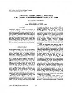
Figure 4 shows how all boolean functions of two variables can be implemented with the neural model. Note that all circuits are pipelined and may have different delays. Circuits of more variables can be obtained by combining these functions. An example is shown in figure 5a. This multiplexer chooses one data bit from two sources (x2 or x3 ) under the control of the select input (x1 ). Figure 5b shows a 3-input AND-gate. Note that this network is smaller than a naive combination of two AND-gates. Another useful example is the majority function (figure 5c) This circuit fires when the majority (two or more) of the inputs received a pulse.

x2 00 x1 0 0

x1

x2 01 x1 0 1

0

x2

x2 10 x1 0 0

x1 x2

x2 01 x1 0 0

x1

x1

3

x2

x2 00 x1 0 1

x2

x1

4

x2

x2 00 x1 1 0

x1 x2

x1

x1

3

x2

x2 10 x1 0 1

+ +

x2

x1

+ +

4

+ + -

4

x2

+

4 +

4

+

x2

x1

1

x2

1

x1

4

x2

x2 10 x1 1 1

x1 + x2

+ +

4

1

x1

4

x2

x2 11 x1 1 0

1

x1

2

x2

x2 01 x1 1 1

2

+ x2

x1

x2 11 x1 0 0

4

x1

2

x2

x2 00 x1 1 1

1

1

x1

x1

4

x2 1

x2 01 x1 1 0

x1

x2 11 x1 0 1

1

x2

x2 10 x1 1 0

1

x2

4

x2

x2 11 x1 1 1

1

x1

1

x1

x1 1

0

x2

Figure 4: All boolean functions of two variables. A ‘1’-input represents a continuous source of pulses. 0 1 1 x1 1

or

x2 0 1 x3 1 1

0 1 0 x1 1

x2 1 0 x3 0 0

0 0 0 x1 0

x1

x3

xor x2 block

0 0 1 x1 1

(a)

x2 0 0 x3 0 0

4

x2

5

x1

x2 0 0 x3 1 0

0 1 0 x1 0

x2 0 1 x3 1 1

0 0 0 x1 0

x2 1 1 x3 0 0

0 0 1 x1 0

x1

x2 0 1 x3 1 1 5

x2

x3 0 0 1 x1 1

0 1 0 x1 1

x2 1 1 x3 0 0

(b)

x2 1 0 x3 1 0

x3 0 0 1 x1 1

x2 1 1 x3 0 0

0 0 0 x1 1

x2 1 0 x3 0 0

(c)

Figure 5: (a) 2-to-1 multiplexer (if (x1 ) then (x2 ) else (x3 ) == (x1 or x3 ) xor (x1 and not x2 )). (b) 3-input AND function. (c) Majority function of three inputs.

2.4

Sequential functions

spike quadrupler

memory loop

4

x

The spike doublers in figure 6 convert a single pulse in a sequence of two pulses (010 −delay→ 0110). The difference is that the right version also can handle consecutive pulses on its input. The left version will convert 0110 into 01010 where the right version converts it into 01110. in

+

+

In

8

Figure 8: Two on/off toggles. Note how the right version makes use of the external input (as in figure 2c).

in +

+

4 out

+

+

8 out

(a)

ticks2 and a spike on the off-input must not arrive 2,3,4 or 5 clock ticks after a spike on the on-input, otherwise the switch will have distorted output.

(b) +

Figure 6: Two spike doublers.

+ + + -+ +

+

on

8

set/reset memory

2

(a)

+ + + -+ +

5

+

set

+

Memories can be made easily with feedback loops of a length equal to the number of bits one likes to store (figure 7a). The smallest possible loop contains four cells (4 bit memory). Memories of an odd number of cells are possible by including a neuron in the loop (as in figure 2b). The content of the memory can be set/reset by injecting a pulse at the appropriate moment. The circuit of figure 7b shows a 5 bit memory with a separate set- and reset-input. The bits are now stored in a double feedback loop.

spike quintuplers

off

Figure 9: An on/off switch.

A simple way to have a constant stream of spikes for specified period is the adjustable timer (one-shot) of figure 10. The input spike is used to turn on an on/off toggle. The same spike turns the toggle back off after being detoured for the desired period. x

reset

(b) +

Figure 7: (a) Simple memory feedback loop. (b) A set/reset memory. Because its six faces are used, the neuron is shown in 3D.

t-1

10

+ on/off toggle

delay

Figure 10: An adjustable timer (one-shot). On/Off toggles (figure 8) make it possible to toggle a continuous stream of pulses on or off. An On/Off switch with separate on- and off-inputs is shown in figure 9. If two spikes arrive at the two inputs at the same time (or with a difference of 1 clock tick) the switch will be on. The minimum time-interval between two spikes on the same input should be 5 clock

The structure in figure 11 can retrieve the (positive3 ) state of a neuron when a spike arrives at the upper input. Only if the state of the neuron is one, a spike 2 This

can be avoided by applying the technique of figure 6b. circuit will not work correctly if the neuron has a negative state. 3 This

1

5

7

9

… B …

2

4

6

8

… A …

In

In

0

1

3

5

7

9

… B …

2

4

6

8

… A …

+

6 Out

3

+

will be emitted on the test output. The neuron preserves its normal function as long as no spikes arrive simultaneously with the test input. Only if the neuron receives spikes during the test the results of the normal operation of the neuron will be affected.

Out

6

0

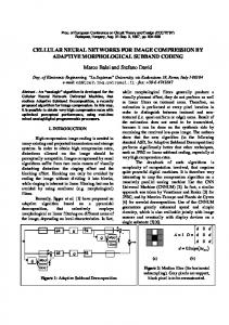
Figure 12: Generate an arbitrary spike train.

test in spike doubler and

(delayed)

3

+

+

+

time: 012345678 target: 100101101

5

+

7 block

5 2 3 6 out

+ +

Out 6

15 3 neuron

in

Fixed spike trains

It is also possible to generate arbitrary spike trains with the CBM’s neural model. With the specific configuration of figure 12 a predefined spike train is produced after receiving a single spike at the input. The principle is simple: Let the pulse propagate through one chain of cells and let it split into a second chain at those points where one wants a spike in the target spike train. Because there are no diagonal connections, two different chains are needed for the spikes on even and the spikes on odd clock ticks. The spike train of the odd chain has to be delayed by one clock tick before it is combined with the spike train of the even chain. There are two ways to implement this as mentioned in 2.2. A simple example is given in figure 13. With this technique it is possible to build modules that can follow a given target spike train for 6864 clock ticks4 . This is remarkably much larger than 70, the result of the genetic algorithm, as mentioned in [5].

3

0

6

8

test out

Figure 11: Test if the state of a neuron is one or zero. The numbers above the arrows indicate the length of the path.

2.5

In

Conclusions

This paper has presented some reusable primitive pulsed neural network structures for the CAM-Brain 4 Because the chains have to be folded into the module, a few bits can’t be generated (5 times 2 bit).

Figure 13: An example of the generation of an arbitrary spike train.

Machine. These basic structures can serve as building blocks for the design of more complex networks. We expect that these networks can form the base of a much more powerful gene pool for the CBM’s genetic algorithm. However, before we can effectively verify this, we shall have to modify this algorithm so that it can take advantage of the higher complexity of these genes.

References [1] M. Korkin, G. Fehr, and G. Jeffery. Evolving hardware on a large scale. In Proceedings. The Second NASA/DoD Workshop on Evolvable Hardware, pages 173–81. IEEE Comput. Soc., July 2000. [2] M. Korkin, N. E. Nawa, and H. de Garis. A “spike interval information coding” representation for ATR’s CAM-Brain machine (CBM). Lecture Notes in Computer Science, 1478, 1998. [3] H. Van Marck and Y. Saeys. Haalbaarheidsstudie van de CAM-Brain computer (dutch). Technical report, S.AI.L, 2001. [4] A. Buller, H. Eeckhaut, and M. Joachimczack. Pulsed Para-Neural Network(PPNN) synthesis in a 3-D cellular automata space. In The 9th Int. Conference on Neural Information Processing (ICONIP’02), November 2002. [5] H. de Garis, A. Buller, T. Dob et al. Building multimodule systems with unlimited evolvable capacities from modules with limited evolvable capacities (MECs). In Proceedings. The Second NASA/DoD Workshop on Evolvable Hardware, pages 225–34. IEEE Comput. Soc, July 2000.