Handling Degenerate Cases in Exact Geodesic. Computation on Triangle Meshes. Abstract The computation of exact geodesics on trian- gle meshes is a widely ...
The Visual Computer manuscript No. (will be inserted by the editor)
Yong-Jin Liu · Qian-Yi Zhou · Shi-Min Hu
Handling Degenerate Cases in Exact Geodesic Computation on Triangle Meshes
Abstract The computation of exact geodesics on triangle meshes is a widely used operation in computer-aided design and computer graphics. Practical algorithms for computing such exact geodesics have been recently proposed by Surazhsky et al (2005). By applying these geometric algorithms to real-world data, degenerate cases frequently appear. In this paper we classify and enumerate all the degenerate cases in a systematic way. Based on the classification, we present solutions to handle all the degenerate cases consistently and correctly. The common users may find the present techniques useful when they implement a robust code of computing exact geodesic paths on meshes. Keywords Exact geodesic computation · Degenerate cases · Robustness
Fig. 1 Geodesic computation with a prescribed source point; points on the mesh are colored according to the geodesic distance to the source point.
reported. In this paper we enumerate all the degenerate cases risen from implementation in [5] and show that in most cases with arbitrarily shaped triangles, the degenerate cases are frequently appears. An example is il1 Introduction lustrated in Fig. 1. The mesh used in Fig. 1 has 2000 faces, 6000 edges and 1028 vertices. The triangles in the An exact geodesic between two points in a 2-manifold mesh are arbitrarily shaped, including both obtuse and mesh is a union of line segments within the mesh which acute triangles. Given a prescribed source point, there connects the two points and is locally length-minimized. are totally 8807 cases handled, in which 2583 cases are The computation of exact geodesic paths on triangle degenerate, about 29.33%. Some degenerate cases are ilmeshes is a widely used operation in computer-aided delustrated in Fig. 4. sign and computer graphics. In geometric computation, degenerate cases will inIn [5], a practical implementation of the DGP algocrease the instability of the generic algorithm. Theoretirithm in [3] is proposed for computing exact geodesics cally, degenerate cases can be handled by using the symfrom a source point to one or all other points efficiently. bolic perturbation schemes [1]. Though it is a powerful In the worst case the DGP algorithm has complexities of tool, this scheme may not be applicable in the computaO(n2 ) space and O(n2 log n) time, while in practice the tion of exact geodesic paths. First, symbolic perturbation algorithm is observed to run in sub-quadratic time. requires exact arithmetic, with which many users are not The implementation in [5] can be regarded as a generic familiar. Second, using symbolic perturbation does not algorithm, i.e., it is guaranteed to be correct with generic solve the degenerate case itself, but an arbitrarily-chosen situation, while how to handle degenerate cases is not nearby general case. Topology-oriented implementation is another way to handle degenerate cases [4]. However, it Department of Computer Science and Technology, only guarantees to output a topology-consistent solution Tsinghua University, P. R. China which may not be the desired topology-correct one. Tel.: +86-10-62784141 Fax: +86-10-62771138 In this paper, to develop a robust and fast exact E-mail: {liuyongjin, zqy, shimin}@tsinghua.edu.cn geodesic algorithm, we present a systematic solution to
2
Yong-Jin Liu et al.
vs
Starting from the source point, the DSP algorithm propagates distance information in a continuous Dijkstralike fashion. When new intervals are created, they are placed in a priority queue sorted by minimum distance back to the source. When an interval is popped from the queue, interval propagation is performed in one of the three cases showing in Fig. 3. The reader is referred to [5] for full details of this algorithm.
σ
y s d0 v0
0
d1
b0
e1
b1
x v2
e0 e2 v1
3 Degenerate cases
Fig. 2 6-tuple representation (b0 , b1 , d0 , d1 , σ, τ ) of the interval.
efficiently handle all the degenerate cases with floating point computation [6]. By doing so, geometric predicates are treated consistently and thus the implemented algorithm is robust.
2 Review of the exact geodesic algorithm We follow the notation in [5] to quick review the DGP algorithm [3]. Shortest paths on mesh are rays emanating from the source vertex along tangent directions. Interior to a triangle, a shortest path must be a straight line. When crossing an edge, a shortest path must be a straight line when the previous face is unfolded into the plane containing the next face. The only vertices (called geodesic vertices below) that a shortest path can pass through are either boundary vertices or the vertices whose total surrounding angle is larger or equal to 2π. The basic idea of the DSP algorithm is to partition each mesh edge into a set of intervals. Refer to Fig. 2. Each interval is encoded by a 6-tuple (b0 , b1 , d0 , d1 , σ, τ ). b0 , b1 are parameters measuring distance along the edge. The unfolded position s of the geodesic vertex is encoded by its distances d0 , d1 to the interval endpoints. A binary direction τ is used to specify the side of edge on which the source lies. σ is the length of the path from s back to the source vs . Given an interval I on an edge e0 , its distance field is propagated across an adjacent face to define new potential intervals on the two opposing edges e1 , e2 . Refer to Fig. 3. Three general cases exist for interval propagation. According to different cases, different new intervals are formed on the opposing edges. If intervals already exist on the opposing edges, the new interval may intersect some old ones. If two intervals intersect with a nonempty region δ, a quadratic equation Ap2 + Bp + C = 0
(1)
is solved to determine a new position p ∈ δ such that the updated ranges of the two intervals I and I 0 are (b0 , p) and (p, b01 ), respectively.
In the exact geodesic algorithm [5], two types of degeneracies occurs in interval propagation: 1. Degeneracies on geometric intersection. Refer to Figs. 3 and 4. These degeneracies rise from the determination of intersection region between the wedge and the line segments e1 and e2 ; 2. Degeneracies on geodesic discontinuities. Due to the numerical errors in floating point computations, the solution of equation (1) often generates small gaps or overlaps between the new resulted intervals; this gives rise to geodesic discontinuities along the intervals on the edge.
3.1 Degeneracies on geometric intersection Basically, there are 5 degenerate cases in this class, as shown in Fig. 4: 1. The position of s lies on edge e0 . This case can happen if the interval is created on e1 in the case of Fig. 3(c); 2. Three points s, b0 , v1 are in a straight line. This makes the new interval on the edge e1 disappear in the case of Fig. 3(b); 3. Three points s, b1 , v1 are in a straight line. This is a symmetric case of case 2; 4. Four points s, v0 , b0 , v1 are in a straight line. This also means that points v0 and b0 coincide. In this case, the new interval on the e1 in the case of Fig. 3(b) must be treated as the new interval on the e1 in the case of Fig. 3(c); 5. Four points s, v1 , b1 , v1 are in a straight line. This is a symmetric case of case 4. Notice that there are some degenerate cases composed of several basic cases. For example, referring to Fig. 4, if three points s, b0 , v0 coincides, the basic degenerate cases 1,2,4 occur simultaneously. Different degenerate cases must awake different procedures to process. Treating degenerate cases in random order will result in catastrophic failures in the algorithm. In Section 4.1, we present a concise decision procedure to properly handle all the degenerate cases.
Handling degenerate cases in exact geodesic computation
3
s
s
y
y d0 0 b0 v0 b’0
d0
d1 I
b1
v2 e2
I’ e1
b’1
(a)
d1
b0
0 v0
x
b1
x v2
e1
(b)
v1
y
s
d1
d0 0 v0
v2
e1
e2
e2
(c)
v1
x
b1
v1
Fig. 3 Interval propagation. (a)One new interval created. (b) Two new intervals created. (c) One new normal interval and two additional intervals (in red) created.
y
y s v0
b0
x v2
e0
b1 e0
v0
e2
e1
y
s
v2 e2
e1
b0
x
b1
x
e0
v0
v2 e2
e1
v1
v1
v1 Case (1)
y
s
(2)
(3)
y
s
b0 b1 x v0 e0 v2 e1 e2
s
b0 e0
v0 e1
b1 x v2 e2 v1
v1 (4)
(5)
Fig. 4 Degenerate cases on geometric intersection; the shaded area indicates the wedge range of b0 → s → b1 .
I’
I’.b0
I’.b1
(a) The new created interval
I
Ii i Inew
Ij
(b) Existing intervals j Inew Ii
Ij
Iupdated = {I 0 , I 1 , · · ·} be the set of updated intervals on e, four degenerate cases may occur: 1. 2. 3. 4.
Tiny intervals appear in I; Two consecutive intervals in I intersects; Two consecutive intervals in I separate by a tiny gap; The geodesic distances at the common endpoint of two consecutive intervals are not the same.
I
inside (c) Preprocessing existing intervals
I I i−1
i
I
j
Iupdated
I j−1
(d) Finally updated intervals
Theoretically, if exact arithmetic is used, these cases will not happen or can be regarded as errors. However, in practice, when float-point computation is used and numerical errors are unavoidable, these cases do occur and we regard them as degenerate cases. The solution to handle these degeneracies is presented in Section 4.2.
Fig. 5 Degeneracies on geodesic discontinuities.
3.2 Degeneracies on geodesic discontinuities After the determination of intersection region between wedge b0 → s → b1 and edges e1 , e2 , new intervals are created. Refer to Fig. 5. Suppose that a new interval I 0 with range (I 0 .b0 , I 0 .b1 ) is created on edge e on which there already exists a set of intervals I = {I 0 , I 1 , · · ·} sorted by positions on edge, I i−1 .b1 ≤ I i .b0 < I i .b1 ≤ I i+1 .b0 . If the intervals I 0 and I i ∈ I have a nonempty intersection region δ = I 0 ∩I i , a quadratic equation needs to be solved to determine the minimal distance for points in δ and update the intervals I 0 and I i along edge e. Let
4 Handling degenerate cases In geometric algorithms, testing degenerate cases relies heavily on the incidence decisions such as whether a point lies on a line or two points coincide [2]. Incidence decisions contribute to geometric predicates. A predicate is a numerical primitive computation whose value impacts the flow of control of an algorithm. To evaluate predicates with float-point computation, we present a systematic solution in the following subsections. The pseudo-code of the overall algorithm is as follows.
4
Yong-Jin Liu et al.
Begin No
s coincides with b0 or b1 Yes Handling new intervals on e1, e2 End (cf. fig. 4.1)
No
s, b0, v1 lie on a same line Yes Handling new intervals on e2 v0, b0 coincide
v1 lies on left side of line s − b0 Yes Handling new intervals on e2
Yes Handling new intervals on e1
No
Yes Handling new End (cf. intervals on e1 fig. 4.2) End (cf. fig. 4.4)
No
s, b1, v1 lie on a same line
v2, b1 coincide
No
Yes Handling new End (cf. intervals on e2 fig. 4.3) End (cf. fig. 4.5)
v0, b0 coincide
No v1 lies on right side of line s − b1 Yes No
Handling new intervals on e1
No Handling new intervals on e1, e2
No End (cf. v1, b1 Yes End (cf. fig. 3b) coincide sym.to Handling fig. 3a) Yes new intervals on e1, e2 Handling End (cf. new intervals fig. 3a) on e1, e2 End (cf. fig. 3c) End (cf. sym. to fig. 3c)
Fig. 6 The flowchart of the decision system to handling degeneracies on geometric intersection.
Algorithm 1 1. Initialize a priority queue Q with a given source point in the mesh; 2. while Q is not empty 2.1. pop off the top element q from Q; 2.2. establish the local system as shown in fig. 3 based on q = (b0 , b1 , d0 , d1 , σ, τ ); 2.3. find the intersection of the wedge b0 → s → b1 and e1 , e2 ; handle the degeneracies using the solution presented in Sec. 4.1; 2.4. update intervals on e1 , e2 and Q using the solution presented in Sec. 4.2; 2.5. if new intervals created 2.5.1. add them into Q; 4.1 Handling degeneracies on geometric intersection Suppose that we implement the vector operation in a C++ class. Given a point (or a vector) p, p.x, p.y, p.z retrieve its three coordinates. p.length() return the value of the vector length. p · q returns the value of the inner product of two vectors p, q. p×q returns the vector of the cross product of p, q. abs(c) returns the absolute value of c. Denote the machine precision by ². Refer to Fig. 3. The following rules consist of incidence decisions: – If (s − b0 ).length() < ², points s and b0 coincide; – If (s − b1 ).length() < ², points s and b1 coincide; – If abs(((s−b0 )×(b0 −v1 )).z) < ², three points s, b0 , v1 lie on a straight line;
– If ((b1 − s) × (v1 − b1 )).z > ², the vertex v1 lies right of the wedge and the new interval will be on the e1 . That means case (a) in Fig. 3 occurs. – If ((b0 − s) × (v1 − b0 )).z < −², the vertex v1 lies left of the wedge and the new interval will be on the e2 . – If ((b0 − s) × (v1 − b0 )).z > ² and ((b1 − s) × (v1 − b1 )).z < −², the vertex v1 lies inside the wedge formed by two rays b0 − s and b1 − s. That means case (b) in Fig. 3 occurs; Given the above rules, our goal is to design a decision procedure that reduce all possible decisions to a set of predicates as few as possible, which also guarantee to output a consist and right decision on choosing the order of different degenerate cases. We present such a nontrivial decision tree in Fig. 6. Given the rules of incidence decisions and the decision tree as shown in Fig. 6, the code that can robustly and consistently handle all the degenerate cases in this class is readily to build.
4.2 Handling degeneracies on geodesic discontinuities Here we present a robust solution to handling degeneracies on geodesic discontinuities. The presented solution may seem unnecessarily complicated at the first glance. However, it not only give us a concise way of programming, but also it makes verification and error estimation possible and easy to realize at each step by providing deterministic status to check. The pseudo-codes handling
Handling degenerate cases in exact geodesic computation
degeneracies on geodesic discontinuities (ref. the Step 2.3 in Algorithm 1) are as follows. Algorithm 2 1. for all I i ∈ I 1.1. let interb0 = max{I i .b0 , I 0 .b0 }, and interb1 = min{I i .b1 , I 0 .b1 }; 1.2. if interb0 < interb1 1.2.1. if I i .b0 < interb0 1.2.1.1. separate I i at interb0; i 1.2.1.2. let Inew = (I i .b0 , interb0) and I i = (interb0, I i .b1 ); i 1.2.1.3. insert Inew into I; 1.2.2. if interb1 < I i .b1 1.2.2.1. separate I i at interb1; i = (I i .b0 , interb1) and 1.2.2.2. let Inew i I = (interb1, I i .b1 ); i into I; 1.2.2.3. insert Inew 2. for all I i ∈ I which completely inside I 0 2.1. update I i and I 0 by solving equation (1); 3. Remove tiny intervals in I; 4. Sew small gaps in I; 5. In I merge neighbor intervals with the same geodesic vertex; 6. (Optional) verification of I if needed.
5
2000 faces, degeneracy rate 29.33%
Given the newly created interval I 0 and a set of already existed intervals I = {I 0 , I 1 , · · ·} on edge e, we first process all intervals in I such that for each interval 5000 faces, degeneracy rate 31.13% in I, it is either completely outside range I 0 or completely Fig. 7 An exact geodesic path over the head model with two inside I 0 . This process is illustrated in Fig. 5c and Step different resolution meshes. 1 in Algorithm 2 serves this need. At Step 2 in Algorithm 2, denote the sorted subset by Iinside whose elements are completely inside the range The biggest advantage of Algorithm 2 is the result of of the new interval I 0 . We update intervals in Iinside in every step is predictable and thus code verification is turn. Given Ii ∈ Iinside and I 0 , a quadratic equation easy to check. is solved. According to the solution, Ii = (Ii .b0 , Ii .b1 ) may disappear or shrink into a smaller interval Iinew = (Iinew .b0 , Iinew .b1 ). In the latter case, we divide interval 5 Results 0 I 0 = (I 0 .b0 , I 0 .b1 ) into two parts, i.e., Inew = (I 0 .b0 , Iinew .b0 ) 0 0 0 and I = (Iinew .b1 , I .b1 ), and insert Inew into I. Then By handling all the degenerate cases consistently and we continue to process Ii+1 with I 0 until all elements in correctly, the implementation of the exact geodesic algorithm [3,5] is very robust. In this section, we present Iinside are processed. Finally, we get an updated interval set I. It is not dif- some testing examples with the models of various disficult to check that given the above rules, the elements in tribution of triangles. In each example, the small green I cannot be intersected to each other. Due to numerical sphere indicates the position of the prescribed source computation, tiny intervals and small gaps may occur. point with which a distance field is built by computRefer to Fig. 5c and Steps 3,4,5 in Algorithm 2, the fol- ing the length of geodesic paths from the source to all other points on meshes. By tracing the gradient of the lowing rules handle these degeneracies: distance field, a geodesic path from the source to a des1. Detect and remove tiny intervals. ∀Ii ∈ I, if Ii .b1 − tination point on mesh is also shown in each example. Ii .b0 < ², merge Ii with Ii−1 or Ii+1 ; In all examples shown here, the degeneracy rate is mea2. Detect and sew small gaps. If Ii+1 .b0 − Ii .b1 < ², let sured by the percentage of degenerate cases over all the Ii+1 .b0 = Ii .b1 be the midpoint of the original Ii+1 .b0 cases. Table 1 summarizes the degeneracies tests on all and Ii .b1 ; the examples. In Fig. 7, a head example with two different resolu3. Merge intervals with the same source point. For any pair Ii and Ii+1 , let the unfolded position of geodesic tion models is presented. Both models consist of irreguvertex be si and si+1 , respectively. If (si −si+1 ).length() lar triangles. On both models, the source and destination < ε, merge intervals Ii and Ii+1 . points are the same and the geodesic paths connecting
6
Yong-Jin Liu et al.
Table 1 Degeneracies tests on all the examples; the degeneracy rate is measured by dividing the degenerate cases resulted from geometric intersection over all the cases. model
face num.
all cases
degeneracy rate
fig7a fig7b fig8 fig9a fig9b fig9c fig9d fig9e
2000 5000 47415 12436 11000 11774 12000 21152
8807 23221 194851 49697 49028 63992 49621 82397
29.33% 31.13% 33.25% 32.40% 29.22% 27.96% 31.41% 35.27%
them are shown. In Fig. 8, the test is performed on the maxplunck head model. This model possesses different mesh resolution over different regions. On this model, a geodesic path crossing regions of different resolutions is shown. These two examples shows that (1) more smaller the triangles are, more degenerate cases occurs; (2) more irregular the triangle distribution is, more degenerate cases occurs. We also test the implementation on a diversity of models with arbitrary triangles. Four typical examples are shown in Fig. 9. These examples show that realworld data is likely to contain a large number of degeneracies. By providing a concise and consistent solution to all the degenerate cases, the users may find the technique presented in this paper useful when he/she implements a robust code to compute exact geodesic over triangle meshes. 6 Conclusions Geometric algorithms are sensitive to degeneracies risen from special positions of several incident geometric objects. Although the general technique [1,4] exists to handle the degeneracies theoretically in any geometric algorithms, certain particular applications permit much more efficient ways to handle degeneracies. In this paper we classify and enumerate all the degenerate cases in the computation of exact geodesics on triangle meshes. Based on the classification, we present a systematic treatment to handle all the degeneracies consistently. We also show by examples that the real-world data is likely to be degenerate. The common users may find the presented technique useful to obtain a robust implementation of the fast exact geodesic algorithm. References 1. H. Edelsbrunner, E. Mucke. Simulation of simplicity: a technique to cope with degenerate cases in geometric algorithms. ACM Trans. Graphics, 1990, 9(1):66-104. 2. C. Hoffmann. Robustness in Geometric Computations. Journal of Computing and Information Science in Engineering, 2001, 1(2):143-155.
Fig. 8 The exact geodesics over the maxplunck head model which possesses different resolution over different regions. The code must be robust against large and small triangles simultaneously existed on a single mesh. The degeneracy rate of this model is 33.25%. 3. J. Mitchell, D. Mount, C. Papadimitriou. The discrete geodesic problem. SIAM J. Comput., 1987, 16(4):647-668. 4. K. Sugihara, M. Iri, H. Inagaki, T. Imai. Topologyoriented implementation – an approach to robust geometric algorithms. Algorithmica, 2000, 27(11):5-20. 5. V. Surazhsky, T. Surazhsky, D. Kirsanov, S. Gortler, H. Hoppe. Fast exact and approximate geodesics on meshes. ACM SIGGRAPH 2005, pp. 553-560. 6. J. Zachary. Introduction to Scientific Programming, Santa Clara, CA : TELOS, 1998.
Handling degenerate cases in exact geodesic computation
7
a b e c d Fig. 9 The computation of exact geodesics over the diverse models with arbitrary triangles.