Hardware/Software Co-design With the HMS Framework - CiteSeerX

Hardware/Software Co-design With the HMS Framework Michael Sheliga Edwin Hsing-Mean Sha

Dept. of Computer Science & Engineering University of Notre Dame Notre Dame, IN 46556

ABSTRACT Hardware/Software co-design is an increasingly common design style for integrated circuits. It allows the majority of a system to designed quickly with standardized parts, while special purpose hardware is used for the time critical portions of the system. The framework considered in this paper performs Hardware/Multi-Software (HMS) co-design for iterative loops, given an input speci cation that includes the system to be built, the number of available processors, the total chip area, and the required response time. Originally, all operations are done in software. The system then substitutes hardware (adder, multiplier, bus) for software based on the needability of each type of hardware unit. After a new hardware unit is introduced the system is rescheduled using a variation of rotation scheduling in which operations may be moved between processors. Experimental results are shown that illustrate the eciency of the algorithms as well as the savings achieved.

i

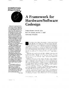
1 Hardware/Software Co-design Introduction The design of computer systems that incorporates both standardized o the shelf processors, or software, as well as specialized hardware is referred to as hardware/software (hw/sw) co-design [9]. Since the complexity and functionality of the computer systems is increasing at a dramatic rate, it is very dicult for custom systems to be designed, built, and tested within an acceptable time period even with the most advanced computer-aided design tools unless standardized parts are used. However, many systems also have time critical parts which must be implemented in hardware. Hence hw/sw codesign is becoming an increasingly important design style. Hardware/Software systems are able to take advantage of standardized processors which have been previously designed and tested to reduce design time and improve reliability. At the same time they use hardware to meet time and area constraints which could not be met by only using general purpose processors. This paper presents several algorithms that perform hw/sw co-design given chip area and timing constraints. Since the nal design consists of one hardware partition and several software partitions it is referred to as the hardware/multi-software, or HMS, system. The HMS system partitions the input speci cation into hardware and software while taking into account the number of inter-partition buses. Scheduling is done in conjunction with partitioning. While this paper is mainly concerned with hardware minimization and partitioning, there are several additional factors that must be considered during hw/sw co-design. Scheduling, pin limitations and bus constraints all contribute to the complexity of the design process. Each of these is considered by our algorithms. As an example, consider the optical wheel speed sensor system shown in Figure 1 (A) which is to be implemented in 100 clock cycles using no more than 40 square units of chip area. As with most systems, this one could be implemented using standardized processors, specialized hardware, or various combinations of both of these. Figure 1(B) shows a design of the wheel speed sensor system that has been implemented solely in software. Note that while the system was designed in only two months, it does not meet the chip area constraints or the timing constraints. Hence, while this design was easiest and fastest to build and test, it is not acceptable. Figure 1(C) shows a second design that has been implemented solely in hardware. The system surpasses both the area and timing constraints by at least 40%. In fact, it is minimum in terms of the AREA  TIME product. However the design cycle time has increased to nine months. In many applications, especially those in which products are sold competitively, such delays are becoming increasingly unacceptable. This is especially true as hardware advances continue to come at faster rates and the eective lifetimes of computer systems are reduced. 1

Input Decoding

Tick to Speed Inversion

FIR Filter

Processor 1

Processor 2 Processor 5

Output Encoding Processor 3

System Constraints Area - 40 Units Time - 100 Cycles

Processor 4

Area - 48 Units Time - 132 Cycles Design Time - 2 Months

(A) (B)

Processor 1

Processor 2

Processor 3 ASIC

Area - 24 Units Time - 52 Cycles Design Time - 9 Months

Area - 37 Units Time - 95 Cycles Design Time - 3.5 Months

(C)

(D)

Figure 1: A) Block diagram of an optical wheel speed sensor system. B)The system implemented in hardware. C)The system implemented in software. D) The system implemented using hw/sw co-design. Figure 1 (D) shows a third design of the system which is implemented in both hardware and software. While the design is not as ecient as the design in (C), and was ready to be used slightly later than the design in (B), it establishes a balance between the two extremes. The implementation in (D) allows the designer to market his product before the competition while also meeting the technical constraints. In addition to the above trade-os, there is also an implicit trade o between the amount of hardware used (and hence the chip area used) and the response time of the nal system. Since specialized hardware adds signi cantly to the design and test cycle time, our algorithms emphasize keeping the hardware to a minimum, providing that time and area constraints are met. Since hw/sw co-design is a new area, relatively little research has been done on actually synthesizing an entire design. Most research has focused on particular aspects of the design process such as creating appropriate abstractions and speci cations of the problem [4, 3], hw/sw interfaces [7, 17], and performance estimation [5, 18]. Other research which has actually synthesized systems has done so for particular types of systems. For instance [16] covers low power systems while [1] considers telecom 2

systems. A customized processor is automatically generated by Holmer and Prangle in [13], however, traditional hw/sw co-design is not performed. Given an input problem, a processor instruction set, data path, and control paths are extracted and a programmable processor is produced. The processor generated is a \combination" of hardware and software. It is a processor geared toward the problem at hand, but which should be able to solve similar problems in an ecient manner. COSYMA [12, 2] performs hw/sw co-design using a simulated annealing partitioning algorithm. As with the HMS system all operations begin in software and are moved to hardware, however, COSYMA assumes a target architecture of one processor, one hardware component, one global bus and one global memory while the HMS system allows a variable number of buses and software units. Furthermore, the HMS system performs scheduling along with partitioning. Gupta and DeMicheli [10, 11] perform traditional hw/sw co-design for reactive systems which have inputs whose arrival times are unknown. Their system, VULCAN II, performs partitioning by examining the inputs for each operation. Operations whose inputs have unbounded delays are called nondeterministic operations, while all other operations are deterministic. If an unbounded delay is caused by waiting for an external input the operation is called an external nondeterministic operation. All other nondeterministic operations are internal operations. Operations are then partitioned into hardware and software largely based upon which of the above classes they are in. VULCAN II performs static scheduling for groups of operations but cannot schedule all nodes since the delay times of some inputs are unknown. Hence it also uses dynamic scheduling. While VULCAN II performs both partitioning and scheduling, there are several important dierences between their system and ours. First their algorithm begins with all operations in hardware and then moves operations to software. Operations may not be moved from software to hardware. In contrast the HMS system begins with all operations in software and then adds hardware units. The HMS system then allows operations to be transferred from hardware to software as well as from software to hardware. A second important dierence is that our system considers a varying number of software components and buses but only one hardware component while VULCAN II presumes their is one system bus, one software component, and multiple hardware components. Perhaps the most crucial dierence is that the HMS system is targeted towards a dierent set of applications. VULCAN II is designed for reactive systems where the arrival time of some inputs are unknown. Therefore VULCAN II uses both dynamic scheduling and static scheduling while partitioning 3

the system. On the other hand the HMS system is meant for iterative loops such as DSP lters in which the arrival times of all inputs are known. Hence it is able to perform a variation of rotation scheduling that allows data to be transferred back and forth between partitions several times. Our system designs single-chip integrated circuit which can be represented as a data ow graph. It begins with an all software implementation and then adds hardware until the area and timing constraints are met. During each iteration of the HMS system three basic steps are performed. First we decide what hardware to add to the system based upon the needability of each type of hardware. The needability is a measure of how often an operation of this type cannot be scheduled due to resource constraints. Operations that are on the critical path are given extra weighting when calculating the needability. The second step is to add the new hardware and transfer operations to it. We present two algorithms to do this. The rst, delayed reallocation, only adds the new hardware, while the second, immediate reallocation, also transfers groups of operations to the new hardware. Groups of operations are chosen based upon how many timesteps may be saved by transferring them, as well as the timesteps saved for the successors of these nodes. The nal step of each iteration compacts the schedule using variable partition rotation, a variation of rotation scheduling that allows nodes to be transferred between partitions. Nodes are transferred to the partition that leads to the best available timestep for all nodes. In addition to these three steps the HMS system also veri es that the bus requirements are met for each rotation. The bus scheduling problem is a variation of the bin packing problem and a modi ed best- t algorithm is used to solve it. Section 2 introduces de nitions and terminology used by our algorithms while Section 3 covers the assumptions of our system and introduces the main ow chart of the HMS system. Section 4 explains the HMS co-design algorithms in detail. Section 4.1 shows how the system calculates the needability of each type of unit while Section 4.1.2 explains how buses are scheduled and allocated. Section 4.2 presents the delayed reallocation and immediate reallocation algorithms. Included in this section is an explanation of variable partition rotation scheduling. Section 5 demonstrates the eectiveness of the algorithm for several input systems. Finally, Section 6 draws conclusions from the results obtained and summarizes our research.

4

2 De nitions and Terminology De nition 1 A Data Flow Graph (DFG) is a node weighted and edge weighted directed graph G = (OP; E ; T ; type; ti; de) where

 OP = foi j 1  i  ng is the set of computation nodes, or operations  E = fel j 1  l  E g, E  OP  OP , is the set of directed edges which de ne the precedences from nodes in OP to nodes in OP

 T = ftk j 1  k  mg is the set of operation types  type(oi), is a function from OP to T representing the type of operation oi  ti(tk ), is a function from T to the positive integers representing the computation time of a node of type k

 de(el ), is a function from E to the nonnegative integers representing the number of delays on edge el

We assume ti(tk ) = 1 8 k for all software operations the remainder of the paper. This unit of time is referred to as one timestep. De nition 2 A Partitioned, Scheduled Data Flow Graph is a DFG Gps = (OP; E ; T ; P ; type; ti; de; part; tsp) where each oi has been assigned to a partition and a timestep in which it starts to execute.

 P = fpj j 1  j  P g is the set of partitions  part(oi) is a function from OP to P representing the partition which operation oi is located in  tsp(oi) is a function from OP to the positive integers representing the timestep in which operation oi is to begin execution

 ti(el ) is a function from E to the nonnegative integers, representing the time it takes to transfer data using edge el

5

All other de nitions are the same as for an unpartitioned, unscheduled DFG. We use the notation eab to denote an edge which begins at node a and ends at node b. Node a is said to be the predecessor of node b while node b is said to be the successor of node a. We assume ti(eab ) = 0 for all edges where part(a) = part(b), and ti(eab ) =  for all edges where part(a) 6= part(b), unless noted otherwise.  is a constant for all edges. We also note that each standardized processor used in the design will correspond to one partition, pj , while the additional specialized hardware will also correspond to a single partition. De nition 3 A Retiming of a DFG is a function from OP to the set of integers. re(oi ) represents the number of delays moved from each incoming edge of operation i to each outgoing edge of operation i during a retiming. If Gr is a retimed version of data ow graph G, then der (euv ) = de(euv ) + re(u) ? re(v) for edge euv . A retiming r is legal if der (e) >= 0 8 e. Intuitively, this means that edges may not have a negative number of delays. Also note that the number of delays in any loop of a DFG must be greater than zero[14]. This property may not be altered by a legal retiming.

3 Main Idea With any hardware/software co-design system it is important to remember what assumptions are made as well as what limitations are placed on the system. We brie y present these as well as the main ow chart of the system in the rst two sections. We then brie y discuss how we decide what hardware to add to the system as well as how we reschedule the DFG once extra hardware has been added.

3.1 Assumptions Our system assumes that a DFG is given and that it is to be scheduled in a given number of timesteps. A limit on the amount of area that may be taken up by the nal design is also given. The hardware used to build the system is of two types. Standardized, or o the shelf, processors may be used to construct the system. Systems constructed in this manner require the least design time. They also require software simulation, test and veri cation, as opposed to hardware simulation, fabrication and veri cation which are assumed to be more time consuming. However, standardized processors tend to be slower and take up more chip area than specialized hardware. Hence, our system attempts to establish a tradeo between design time compared to chip area and speed. 6

For the remainder of the paper we assume that the standardized hardware consists of one type of processor, while the specialized hardware consists of adders and multipliers. These assumptions simplify the explanations of how our system works as well as its implementation, however they may easily be modi ed. The chip area taken up by adders, multipliers, standardized processors, and global buses is also given. The area taken up by intra-partition buses is assumed to be negligible. It is assumed that hardware runs at a faster rate than the software and that this rate is xed for all operation types. Hence if hardware multipliers are 50% faster than software multipliers then hardware adders are 50% faster than software multipliers. While hardware may be any percentage faster than software in our system, numbers that result in low integral fractions when comparing software cycles to hardware cycles are used to simplify the examples presented. In cases where there may be confusion between software timesteps and hardware timesteps, \timesteps" refers to software timesteps, while \hardware timesteps" refers to hardware timesteps. In the case of time delays for inter-partition data transfers, all data takes one software timestep, not one hardware timestep.

3.2 The Main Algorithm of the HMS System Figure 2 presents the main algorithm of the HMS system. The details of each subroutine are explained in Section 4. We begin by attempting to implement the entire system using standardized processors. We use as many processors as the chip area allows, and schedule the system using list scheduling. If the system cannot be scheduled in the required amount of time, the algorithm begins to add specialized hardware. The subroutine Most Needed Hardware is used to determine what type of hardware is to be added. If adding a unit of hardware violates the chip area constraint a standardized processor is eliminated and replaced by an equivalent amount of specialized hardware. The additional specialized hardware is equivalent to the standardized processor in that both may perform the same number of operations in a given time if both are fully utilized. For example, if the standardized processor being eliminated from the system contained six adders and two multipliers, and hardware was twice as fast as software, then three hardware adders and one hardware multiplier would be added to the system. We then use either delayed reallocation or immediate reallocation to reschedule the data ow graph. Both of these use variable partition rotation, a variation of rotation scheduling in which operations may be transferred between partitions. We continue this process until the time constraint is met. The algorithm used was chosen since it permits the maximum amount of o the shelf hardware to be used, thereby reducing design time. 7

ALGORITHM MAIN HMS (DFG, Time Desired, Total Chip Area) Input : a DFG Time Desired: The maximum time. Total Chip Area. The Maximum Design Area Output : A Scheduled Hardware/Software Design

begin while (Chip Area Used < Total Chip Area) Add Standard Processor( ); end Time Required ? List Schedule( ); while (Time Required < Time Desired) New Unit Type ? Most Needed Hardware( ); AddNewUnit(New Unit Type); if (Chip Area Used > Total Chip Area) then

Remove Standard Processor( ); Add Equivalent Hardware( ); end if (Algorithm == Delayed Reallocation) then Time Required ? V ariable Partition Rotation( ); else if (Algorithm == Immediate Reallocation) then Move Operations to New Hardware( ); Obtain Legal Schedule( ); Time Required ? V ariable Partition Rotation( );

end end end

Figure 2: The HMS algorithm.

8

3.3 Hardware Addition During the design process new units of hardware (adders, multipliers, buses, etc.) are added to the system. We must determine what type of hardware to add. In order to do this the needability of each type of hardware is determined. The needability of a type of hardware is a measure of how often the system would like to schedule an operation of this type, but cannot due to resource constraints. The type of hardware with the greatest needability is added to the system.

3.4 Rescheduling When new hardware units are added to the system rescheduling is done to see if the system's time constraint can be met. Two algorithms are used to reschedule the system after a new unit of hardware is introduced. Both use a variation of rotation scheduling [6] in which operations may be moved between processors. The rst algorithm, called delayed reallocation, only allows operations to be transferred during rotation scheduling. Transferring operations in groups may be advantageous, especially when the new hardware is faster than the existing hardware. The second rescheduling algorithm, immediate reallocation, transfers operations to the new unit of hardware as soon as it is inserted. Since the new hardware unit has no operations scheduled for any timestep, operations may easily be transferred in groups. As many operations as possible are transferred to the new hardware unit. After operations have been transferred to the new hardware unit unallocated resources will exist in the software, therefore delayed reallocation must still be done in order to maximize the system throughput.

4 Description of Algorithms 4.1 Hardware Addition 4.1.1 Functional Unit Addition When the desired time constraint cannot be met using the current hardware we must use additional hardware. In order to determine what type of hardware to add our algorithm considers the needability, Ntk , of each type of hardware (adder, multiplier, bus, etc.). Intuitively, the needability is an estimation of how often this type of unit is needed but unavailable in the current schedule. In order to calculate the needability of each type of hardware, we de ne partially scheduled DFGs, 9

hw constrained operations and hw constrained critical path operations. Given a scheduled DFG, a partially scheduled DFG at timestep ts is a DFG where operations for which tsp(oi ) < ts are schedule at tsp(oi ) while other operations are not assigned a timestep. An operation oi is a hw constrained operation at timestep ts with respect to a partially scheduled DFG if and only if operation oi could be scheduled at timestep ts but is not in the scheduled DFG due to hardware constraints. Similarly, operation oi is a hw constrained critical path operation at timestep ts if it is a hw constrained operation and the longest path originating at it and terminating at an output node is maximum for all nodes that have not been scheduled in the partially scheduled DFG at timestep ts. Note that these de nitions only depend on the current schedule, not the scheduling algorithm used.

As an example consider Figure 3. Figure 3 (A) shows an example DFG which has not been scheduled, while Figure 3 (B) shows the same DFG after it has been scheduled presuming that 2 adders and 1 multiplier are available. Node 1 could be scheduled in timestep 1 if an additional adder was available. Therefore node 1 is a hw constrained operation. Similarly node 2 could be scheduled in timestep 2 if an additional multiplier was available. Node 2 is also on the critical path at timestep 2, therefore it is a hw constrained critical path operation. By not scheduling node 2 in timestep 2, the length of the schedule is guaranteed to increase. Notice that node 3 is not a hw constrained node, even though it could be scheduled in timestep 3 if unlimited resources were available during scheduling. This is because not all of node 3's predecessors (node 2 in this case) have nished executing in Figure 3 (B) until the end of timestep 3. A similar analysis holds for hw constrained critical path nodes. They are only hw constrained critical path nodes given that they are part of the longest path of unscheduled nodes at this timestep.

P

The needability of operation type tk is de ned as Ntk = Wtk  timesteps (Whw  CHWtk ;ts + ts=1 Wcp  CCPtk;ts), where Wtk is a weighting factor related to the chip area that a unit of type tk takes up, Whw is a weighting factor for hw constrained operations, and Wcp is a weighting factor for hw constrained operations that are on the critical path. CHWtk ;ts and CCPtk ;ts are simply the number of hw constrained and hw constrained critical path operations of type tk at timestep ts. The needability of buses is de ned similarly and is explained further in Section 4.1.2. As an example let us assume Wadder = 7, Wmult = 5, Whw = 1, and Wcp = 1 in Figure 3(B). Wadder is greater than Wmult to re ect the fact that multipliers take up more chip area than adders. Hence we are less hesitant about increasing the number of adders. In Figure 3, Nadder = Wadder  P4ts=1(Whw CHWadder;ts+WcpCCPadder;ts). Noting that CHWadder;ts = 0 for ts 6= 1, CHWadder;1 = 10

= Multiplier

= Adder

Timestep 1

1 2

2

3

3

1

2

4

3

(A)

(B)

Figure 3: A) A sample DFG. B) The scheduled DFG presuming two adders and one multiplier. 1, and CCPadder;ts = 0 8 ts, we have Nadder = Wadder  (Whw  CHWadder;1 ) = 7  (1  1) = 7. Similarly CHWmult;ts = 0 for ts 6= 2, CHWmult;2 = 1, CCPmult;ts = 0 for ts 6= 2, and CCPmult;2 = 1. Hence Nmult = Wmult  ((Whw  CHWmult;2 ) + (Wcp  CCPmult;2 )), = 5  ((1  1) + (1  1)) = 10. The larger value of Nmult compared to Nadder points out that it would be more helpful to increase the number multipliers in the system than the number of adders. Notice that increasing the number of multipliers enables the system to be scheduled in 3 timesteps, however, no increase in the number of adders will be helpful for this system.

4.1.2 Bus Addition Before we begin to discuss the bus scheduling algorithm used as part of the bus needability algorithm we must discuss the data transfer model used. As discussed in [15] there are many dierent ways to model data transfers. First, we must decide how long data transfers take. As noted in Section 2 we assume that all inter-partition data transfers take one time unit and all intra-partition data transfers are done between clock cycles. A second factor to consider is that of when data is transferred. One model of data transfers assumes that all data is transferred as soon as it is calculated. While this model greatly simpli es the calculation of bus statistics, it is inecient since extra buses may be needed for data transfers that could be delayed. A second model of data transfer assumes that data may be transferred 11

at any time between when it is generated and when it is used. We refer to this as the exible transfer model. While this model is more realistic, it can be shown that optimizing data transfers for it is NP-hard [8]. We use the exible transfer model for the remainder of the paper. The needability of buses is similar to that of hardware units. For each timestep we calculate the number of nodes that cannot be scheduled at an earlier timestep due to bus constraints. We weight the nodes that are on the critical path, and sum a weighted count of these numbers over all timesteps. P Hence Nbus = Wbus timesteps (Whw  CHWbus;ts + Wcp  CCPbus;ts ). If Nbus is greater than Ntk ts=1 for all k operation types, then an additional bus is inserted instead of additional hardware. However it is much more dicult to determine when a node may not be scheduled due to bus constraints than it is for hardware constraints. This is due to the fact that bus transfers at the current timestep depend upon bus transfers from other timesteps. Hence, a proposed schedule for the entire graph is used as input to the bus scheduling algorithm. The bus scheduling algorithm then generates a schedule for the data transfers, or a result that indicates such a schedule was not found. The main

ow of this algorithm is shown in gure 4 and is applied when rotating a node (to check enough buses are available for the resulting schedule) as well as for the calculation of Nbus . It should be noted that this algorithm is designed for systems with data transfers of variable length, not only data transfers that take one timestep, as we have assumed in the rest of the paper. The spacing of a data transfer is a measure of the number of timesteps between it and the other data transfers on the bus. It is desirable to schedule each data transfer so that it has zero spacing. Leaving a single unused timestep for a bus makes it dicult for the bus to be used in this timestep. Leaving two or more consecutive timesteps makes it more dicult for the bus to be used eciently as compared to no timesteps but less dicult as compared to a single timestep. We de ne S 1TR;BUS;TS as the number of timesteps between the beginning of data transfer TR and the end of the last data transfer on bus BUS if the data transfer is begun at timestep TS . S 2TR;BUS;TS is de ned as the time between the end of data transfer TR and the start of the next data transfer on bus BUS if the data transfer is begun at timestep TS . We then combine S 1 and S 2 using the formula S = X (S 1)X (S 2) + X (S 1) + X (S 2), where X (S 1) = 0 if S 1 = 0 and X (S 1) = S11 otherwise. X (S 2) is de ned similarly. STR is the smallest STR;BUS;TS for all bus/timestep combinations for the data transfer under consideration. The data transfer (or group of data transfers in case of a tie) with the smallest STR is then chosen. The length of a data transfer is the number of timesteps the data transfer takes (all data transfers are assumed to take integral length). The exibility of a data transfer is the number of timesteps in 12

ALGORITHM BUS SCHEDULING (DFG) Input : A Proposed Node Schedule with a Set of Data Transfers The Number of Buses Output : A Bus Schedule for the Data Transfers Or an Indication that No Schedule was Found.

begin (L ? All Data Transfers) while L 6= NULL

Assign Forced(); /* Choose Transfers with Best Spacing */ for Each Transfer TR in L STR = Spacing(TR);

end

L ? Transfers With Best Spacing(L); /* Choose Transfer with Worst Flexibility */ for Each Transfer TR in L FTR ? Flexibility(TR); 0

0

end

L ? Transfers With Worst Flexibility(L ); /* Choose Transfer with Longest Length */ for Each Transfer TR in L LETR ? Length(TR); end Transfer Chosen ? Longest Transfer(L ); Assign Transfer(Transfer Chosen); L ? L ? Transfer Chosen 0

00

00

00

end end

Figure 4: The bus scheduling algorithm.

13

which a data transfer can be scheduled divided by its length. Data transfers with low exibility have fewer timesteps to be scheduled in so we schedule these transfers rst. Hence, among data transfers with the same spacing, transfers with the least exibility are chosen rst. Likewise, among transfers with the same spacing and exibility those with the largest length are scheduled rst. Large data transfers are the hardest to \ t" into an existing schedule while small data transfers may more easily be scheduled around existing data transfers. As a simple example consider the data transfers in Figure 5(A). Data transfer A takes one timestep and is to be transferred between the beginning of timestep 4 and the end of timestep 5. Its length is 1 while its exibility is 12 . Presuming no data transfers have been assigned buses and noting that all data transfers must be completed by the end of timestep ve, if transfer A is scheduled in timestep 4 using bus 1, S 1A;1;4 = 3 and S 2A;1;4 = 1. This re ects the fact that bus 1 has three unused timesteps between it and the end of the previous data transfer on this bus (or the rst possible transfer time which is one in this case), and one timestep between its end and the next data transfer on this bus (or the last possible time at which data transfers may end in this case). Similarly S 1A;1;5 = 4 and S 2A;1;5 = 0 if transfer A is scheduled in timestep 5 using bus 1. Data transfer B takes 2 timesteps and may be transferred any time between the end of timestep 1 and the end of timestep 5. Its length is 2 while its exibility is 25 . S 1B;1;1 = 0, S 2B;1;1 = 3, S 1B;1;2 = 1, S 2B;1;2 = 2, S 1B;1;3 = 2, S 2B;1;3 = 1, S 1B;1;4 = 3, and S 2B;1;4 = 0, The other data transfers are de ned similarly. We wish to schedule transfers A through I on buses 1, 2 and 3. The algorithm begins by assigning those data transfers which are forced to be scheduled in certain steps. This is done in subroutine AssignForced in gure 4. For example data transfer C must begin at the end of timestep 1 while data transfer F must begin at the end of timestep 3. Transfers C and F are shown in Figure 5 (B) using solid circles. Subroutine AssignForced assigns buses to data transfers using the same spacing concept that is presented below. Next we calculate the spacing, S , for each data transfer. S 1A;1;4 = 2, S 2A;1;4 = 1 and SA;1;4 = X (2)X (1) + X (2) + X (1) = ( 21 )(1) + 12 + 1 = 2. Similiarly S 1A;1;5 = 3, S 2A;1;5 = 0 and SA;1;5 = X (0)X (3) + X (0) + X (3) = (0)( 13 ) + 0 + 13 = 13 while S 1A;2;5 = 0, S 2A;2;5 = 0, SA;2;2 = 0, S 1A;3;4 = 3, S 2A;3;4 = 1, SA;3;4 = 1 32 , S 1A;3;5 = 4, S 2A;3;5 = 0, SA;3;5 = 14 , and SA = 0. These results show that placing data transfer A on bus 2 in timestep 5 results in the best spacing of zero. Similiarly SB = 0; SD = 0; SE = 0; SG = 21 ; SH = 1; andSI = 31 . Therefore data transfers A; B; D and E have the best spacings all of which are 0. Hence L = A; B; D; E . Next the exibility of A; B; D and E are calculated. FA = 2; FB = 52 , FD = 23 , and FE = 5. Since FD is the smallest node D is chosen and is 0

14

Transfer Length

A

B

C

D E F G

H I

Bus

1

2

1

2

1 2

Timestep

1 2

3

1

2

3

Timestep

C

1

1

2

2

3

3

4

4

5

5

F

(A)

1

Bus

2

(B)

3

Timestep

2

3

Timestep

C 1

1

Bus

D

C 1

D

G

B

2

2

F

F

3

3

H

4

I

4

E

5

A

5

(C)

(D)

Figure 5: A) The Data Transfers B) Buses Assigned After Assign Forced() is Called C) The Assignments After One Iteration D) The Final Assignments

15

scheduled starting at timestep 1 on bus 2, which were the timestep/bus combination that resulted in a spacing of 0. The system after transfer D has been assigned is shown in Figure 5 (C). In the next iteration data transfer SB has increased to 12 leaving SA = SE = 0 as the minimum spacing. Since FA is less than FE transfer A is scheduled next. Similiarly transfers I; G and B are assigned at which point transfers H and then E are set via Assigned Forced. The system with all data transfers allocated is shown in Figure 5 (D).

4.2 Scheduling When new hardware units are added to the system, rescheduling is done to see if the system's constraints can be met. Two algorithms are used to reschedule the system. The rst, delayed reallocation, only allows operations to be moved between processors during rescheduling. The second, immediate reallocation, allows operations to be transferred between partitions as soon as the new unit of hardware is added as well as during rescheduling.

4.2.1 Delayed Reallocation Delayed reallocation uses variable partition rotation, a variation of rotation scheduling, to reschedule the graph after new hardware is added. Rotation scheduling, which was developed by Chao, LaPaugh and Sha in [6], consists of retiming a scheduled DFG in order to obtain a DFG with a shorter schedule. Figure 6 (A) shows an example DFG while Figure 6 (B) shows a possible initial schedule for the DFG. In (A) the short thick lines on edges indicate delays. We assume that data transfers between partitions take 1 timestep. During rotation scheduling nodes are rotated down and then pushed up to a new position. Rotating down a node corresponds to retiming the original DFG by moving one delay from all input edges of the node to all output edges of the node. Since rotating a node or group of nodes is equivalent to retiming the original DFG all edges terminating at a node which is being rotated must contain at least one delay. As an example, rotation of nodes A and B is equivalent to pushing the delays on edges terminating at nodes A and B (eDA ; eFB ) to the edges originating at nodes A and B (eAC ; eBD ). When nodes A and B are pushed up we look for a new timestep to place them into. During normal rotation scheduling nodes may not change partitions. Therefore node A is pushed up to timestep 6. Placing node A in timestep 6 does not violate the dependency between node A and any of its predecessors. Notice that node A cannot be placed into timestep 3, even though timestep 3 is unused 16

Software Partition 1

Partition 1

Software

Partition 2

Partition 1 Timestep

A

1

A

B

C

D

2

4

E

5

F

G

F

D

A

B

2

C

D

3

3

E

1

B

C

Partition 2

Timestep

Partition 2

4

E

5

F

6

A

G

G

6

B

7

(B)

(A)

(C)

Software Partition 1

Hardware

Partition 2 Timestep

Timestep 1

A

B

Partition 2

2

C

D

3

1

Software Partition 1

2 3

Timestep 1

A

B

2

C

D A

3 4 5 6

E

4

A

4

E

5

F

6

B

5

C

6 7 8

F

7

B

8

G

9 10 11

G

D

12

9

(D) (E)

Figure 6: A) A partitioned DFG B) A possible schedule C) A single down rotation without changing partitions D) A single down rotation using variable partition rotation E) A second down rotation with new hardware added

17

in partition 1, since node A must begin at least 1 timestep after node D is nished executing. Similarly node B is placed into timestep 7. The new schedule in which nodes A and B have been rotated is shown in Figure 6 (C). The copies of nodes A and B above the thick black line this is between timesteps 1 and 2 indicate that nodes A and B are now part of the prologue of the system, in addition to being part of the repeating, static schedule that is shown for timesteps 2 to 7. Delayed reallocation uses a variation of rotation scheduling in which nodes may be transferred between partitions to reschedule operations on the new hardware. This process is referred to as variable partition rotation. During variable partition rotation nodes may be transferred between partitions as long as changing partitions does not result in a later schedule time. As an example consider Figure 6 (D), in which the same rotation as in (C) is shown. Node A, which was rotated to timestep 6 in (C), may now be rotated to timestep 3 if it is placed in partition 2. Similarly, node B, which was rotated to timestep 7 in (C), may now be placed into timestep 6 if placed into partition 1. Notice that after variable partition rotation the DFG may be scheduled in 5 timesteps, while it required 6 timesteps after normal rotation scheduling. During each down rotation of the variable partition rotation routine the algorithm in Figure 7 is applied. Let us consider the down rotation algorithm in more detail. During each rotation we rotate down all nodes that are in the rst timestep. These nodes are placed in list L. For each node in L we calculate the best timestep that it can be pushed up to by using the subroutine Best Timeslot. We then choose the nodes that may be scheduled the earliest and place them in list L . If there is more than one node in L , we choose the node from L which would be scheduled the latest if it were not placed in this timestep. The subroutine Second Best Timeslot is used to calculate the second best timestep that a node could be scheduled in. Once we have chosen the best node from L we decide which partition to place it into. In most cases this is trivial since it may only be placed into one partition and still be scheduled as soon as possible. However, in situations where the best node may be scheduled at the same time in two or more partitions, the subroutine Percentage Used is used to calculate the percent of timesteps currently used for each of these partitions. The partition with the least percent of timesteps used is then chosen. Once we have chosen what node to rotate, what timestep to place it into, and what partition to place it into, we rotate the node and remove it from list L. This process continues until rotating down all nodes of the DFG does not result in a change in the schedule length. Hence the entire graph may need to be rotated down several times before the minimal schedule is obtained. 0

0

0

0

As an example consider Figure 6(E), in which a new, faster hardware unit has been added to the system. The hardware is 50% faster than the software. By 50% faster, it is meant that each hardware 18

ALGORITHM VARIABLE PARTITION DOWN ROTATE (DFG) Input : A DFG Output : A DFG which has been rotated down once. begin (L ? Nodes in First Timestep(DFG)) while (L =6 NULL) /* Choose Nodes That May Be Pushed Up To the Highest Timeslot */ for Each Node in L TNode = Best Timeslot(Node); end L ? Nodes With Best Timeslot(L); /* Calculate Where Node Would Be Placed If Not In this Timeslot */ for Each Node in L TNode ? Second Best Timeslot(Node); end Node Chosen ? Node With Worst Timeslot(L ); Timeslot Into ? Best Timeslot(Node Chosen); /* Decide What Partition to Place the Node In */ for All Partitions For Which Node Chosen May Be Placed into Timeslot Into UsedPartition ? Percent Used(Partition); end Partition Chosen ? Least Used Partition(); Rotate It(Node Chosen; Timeslot Into; Partition Into); L ? L ? Node Chosen end end 0

0

0

Figure 7: The variable partition down rotation algorithm. functional unit executes three operations in the time that each software functional unit executes two operations. We now use variable partition rotation to rotate down nodes C and D from Figure 6(D). Node C is scheduled rst since it may be pushed up to (software) timestep 4 while node D may not be scheduled until timestep 8. Node C is placed into timestep 4 in partition 2. Next node D is rotated. Since both nodes B and G are predecessors of D, it may not be scheduled in timestep 7 in either partition 1 or 2. Hence we must decide which partition to place it into. We may place it in partition 1 or 2, in which case it will nish at the end of timestep 8, or in the hardware in which case it will nish at the same time. The hardware is chosen in this case since it is the least used of the three partitions.

4.2.2 Immediate Reallocation Immediate reallocation consists of three steps, moving operations to the new hardware, obtaining a legal schedule, and variable partition rotation. The rst step, moving operations to the new hardware, takes place as soon as a new unit of hardware is added to the system. During this step groups of operations 19

Hardware

Software

= Multiplier

Timestep

Timestep

= Adder Software 1 Multiplier 2 Adders

1

1

2

5

2

3

6 3

4

Hardware 1 Adder 33% Faster

1

4

5

1

1

2

2

4

3

3

5

4

4

2

5

3

6

(C)

(B) (A)

Software

Timestep

1

2 3

Software

Hardware

Timestep

5

Hardware

Timestep

Timestep

1

1

2

2

3

3

4

4

3

5

5

4

6

1

1

1

2

2

2

6

4

3

3

4

4 5

6 5

(E)

(D)

Figure 8: A) Key. B) The scheduled DFG. C) The scheduled DFG with four nodes selected to move to the new adder. D) The scheduled DFG after four nodes have been moved to the new adder. E) The nal DFG after pushing down nodes 5 and 6 and variable partition rotation. are transferred to the new hardware. As many groups as possible are transferred, with the criteria for deciding what groups to be transferred explained below. Since transferring groups of nodes may result in new communication delays that may lead to an illegal graph, some nodes may need to be \pushed down" in order to obtain a legal schedule. This is done in the second step of immediate reallocation. Finally, since the software that the operations were transferred from will now have unused hardware, variable partition rotation is used to nd a shorter schedule in the third step of immediate reallocation. Since the new hardware unit is faster than the software that is already in place, it may be bene cial to transfer groups of operations to the new hardware. As an example, consider Figure 8 (B) which shows an example DFG that has been scheduled on a standard processor which has 2 adders and 1 multiplier. It has been decided to add an adder which is 33% faster than the standard processor to the system. 20

Figure 8 (C) shows the same gure but with the extra adder inserted in the system. In (C) a group of four nodes have been selected to be transferred to the new adder. By transferring four nodes at a time we may \save" an operation since four operations may now be t into three (software) timesteps. Figure 8 (D) shows the DFG after the four nodes have been put into three timesteps and the connections between nodes in the hardware and the standardized processor reestablished. Notice that node 5 cannot be scheduled in timestep 2 as it was in (B) since we assume data transfers between dierent partitions take 1 timestep. Therefore, in (D), nodes 5 and 6 are not scheduled. This is denoted with a dashed line for nodes 5 and 6 and their edges. They will be rescheduled during the second step of immediate reallocation using a simple scheduling algorithm that will \push them down" to the next available timestep so that a legal schedule may be obtained. In this case nodes 5 and 6 may be pushed down to timesteps 3 and 4. Note that when we are obtaining a legal schedule we only push down those portions of the system that are not legal. The whole system is not rescheduled. While we have managed to save an addition by using the faster hardware, we have been forced to delay the execution of nodes 5 and 6 by one time unit. Hence, there is a tradeo when moving nodes to the new hardware. We will decrease the time it takes for some operations, but others may increase. When transferring groups of operations we look for those whose successors may be scheduled earlier if the proposed transfer takes place. After obtaining a legal schedule, variable partition rotation, as explained in Section 4.2.1, is used to arrive at the nal schedule. Figure 8 (E) shows the nal DFG after variable partition rotation. The nal DFG takes four timesteps to execute while the original DFG took ve timesteps. Let us examine the steps of immediate reallocation in more detail. The rst step of immediate reallocation involves transferring nodes to the new hardware. In order to do this we rst decide what nodes to transfer. If the hardware is P% faster than the software at least 100 P + 1 operations must be transferred to the hardware in order to save an operation. For example, if the hardware is 33.3% faster than the software, then 33100:3 + 1 = 4, operations must be moved to the hardware in order to save a timestep. In order to decide what operations to transfer we calculate the time dierential, TD that results from transferring dierent groups of operations. The group of nodes with the greatest time dierential is transferred to the new hardware. Three factors are considered when calculating the time dierential: the number of operations transferred to the new hardware, Ot , the number of operations saved, Os , and the saved successor time of each path aected by the transfer, sti. The time dierential is de ned 21

Pi=1 sti + Os=Ot . as TD = successors 

The term Os=Ot is a second-order term used to resolve ties when the saved successor times are equal. Ot is simply the number of operations transferred to the new hardware. Os is the number of =Ot (tsp(ok )). In other words operations transferred to the new hardware for which tsp(oi) = maxkk=1 Os is the number of operations that are scheduled in the greatest timestep of all operations being transferred.  is a constant which is set large enough (approximately 10) so that the term Os=Ot < 1. This ensures that this term will only make a dierence when the sum of the saved successor times are equal. Intuitively, this term represents the percent of operations transferred to the new hardware that have nished executing at an earlier timestep. The saved successor time represents the number of timesteps that the successors of nodes being transferred could be moved up if unlimited hardware were available. We use the notation tse(oi ) to denote the timestep which operation i (a successor of one of the nodes being transferred to the new hardware) would be scheduled at if unlimited hardware were available given that the nodes transferred to the new hardware have been scheduled. Hence sti = tse(oi )old schedule ? tse(oi )new schedule. As an example consider Figure 9. As noted in (A) the new hardware, an adder, is 50% faster than the standardized processor. Hence we must transfer at least 100 50 + 1 = 3 operations to the adder in order to save a timestep. First let us consider transferring nodes 2, 3 and 5 to the new hardware (Ot = 3). If this were done, node 2 would have to be delayed 1 time unit since it would be in a dierent partition than node 1. Furthermore, node 4 would be delayed an additional time unit because of the data transfer between nodes 2 and 4. Hence st4 = ?2. Similarly, node 8 would need to be delayed two timesteps since the data transfer between it and node 3 would take an additional timestep. On the other hand we would save one time unit by scheduling nodes 2, 3, and 5 on the faster hardware (Os = 1). However, we would also lose one unit of time on the transfer of data from node 5 to node 6, Hence st6 = ?1 and st8 = ?2, and if  = 10, 29 DT = 110=3 + (?2 + ?2 + ?1) = ?4 30 . Overall, we save one operation by moving three nodes but we increase the length of three paths by doing so. Therefore, nodes 2, 3 and 5 are likely not a good choice. In general, nodes that have input that will not be available at the timestep they are currently scheduled in if they are moved to a dierent partition, such as node 2 in this case, are not a good choice . These nodes cannot be scheduled on the faster hardware until one timestep after they were previously scheduled due to the delay associated with transferring data between partitions. As a second example let us consider transferring nodes 1, 2 and 3 to the hardware. In this case all 22

Software Timestep

= Multiplier

1

= Adder

2

Software 1 Multiplier 2 Adders

3

1

4

2

Hardware 1 Adder 50% Faster

3

4

5

8

6

5 6

7

5 11

8

7

9

(A)

9

10

(B)

Hardware

Software

Timestep

Timestep

Timestep

Timestep

1

1

1

1

Hardware

Software

2

2 2

3

3 4 5

1

4

2

5

3

3

3 4

6 7

4

2

5

4

8

9

9 10

6

7 8

5

6

8

(C)

7 9

12

10

2

5

3

6

5

7 8

7

9 10

7

11

11

5 11

4

6

8 6

1

8 9

5 11

(D)

12

9

10

Figure 9: A) Key B) The scheduled DFG. C) The scheduled DFG with three nodes moved to the new hardware. D) The scheduled DFG with six nodes moved to the new hardware. 23

predecessors of node 1 nish executing at least one time unit before node 1 begins executing. Therefore there is no delay associated with moving node 1 to the adder. For nodes 1, 2 and 3 we nd that Ot = 3, 29 Os = 1, pt4 = ?1, pt5 = 0 and pt8 = 0, hence DT = ? 30 . In this case we delay the scheduling of one successor by one time unit. By examining all other combinations we nd that this is the best combination of operations to transfers. The negative value of DT indicates that we force some nodes to be scheduled later rather than sooner. While this is undesirable, it is normally the case with the rst group of nodes transferred to the new hardware since two inter-partition delays are associated with the rst transfer. We next attempt to transfer 3 more nodes. In this case nodes 5, 6, and 7 are the best choice with a DT of 110=3 + (0 + 1 + 1) = 2 301 . The DFG with nodes 5, 6, and 7 transferred to the new hardware is shown in Figure 9 (D). Both nodes 9 and 10, which are successors of node 7, could be moved up one timestep. Note that the other predecessor of node 9, node 11, is ignored since it is not clear what eect rescheduling will have upon it. While we were forced to delay node 4 by one time unit when transferring nodes 1, 2 and 3, we were able to move nodes 9 and 10 up one time unit when transferring nodes 5, 6 and 7. This is a common result of transferring nodes to the new hardware. The rst transfer will often result in other nodes being delayed while successive transfers will result in other nodes being scheduled sooner. This process is continued until no more groups of nodes can be transferred. The second step of immediate reallocation, obtaining a legal schedule, is done using a simple algorithm that \pushes down" illegal nodes. For example, in Figure 8 (D) scheduling node 5 in timestep 2 is illegal. It may not be scheduled in timestep 2 since the data from node 1 is not available until timestep 3. Therefore node 5 is pushed down to the next timestep with an available adder. The process is repeated for all descendants of node 5 which are also illegal. In this case node 6 is pushed down from timestep 3 to timestep 4. Note that in some cases a node may not be able to be scheduled in the available number of timesteps. In such a case the length of the schedule is increased by one. The third step of immediate reallocation, variable partition rotation, is the same as used in delayed reallocation and is explained in Section 4.2.1.

5 Experimental Results This section presents the experimental results for several lters. We rst show detailed results for the delayed reallocation algorithm. After presenting the results we brie y explain what input systems were used to generate them and then analyze the results. Further results are then presented for a variety 24

Number of Units CPU BUS ADDERS MULTS AREA 2 1 0 0 115 1 1 0 120 1 1 1 1 82 1 2 1 87 1 3 1 92 1 3 2 104 0 3 2 39

Results TS TT 80 12 72 11 63 9 48 0 42 0 39 0 39 0

Area Desired = 120: Time Steps Desired = 39 CPU Area = 50: Bus Area = 15 Hardware Timesteps per Operation = 3 Minimum Possible Timesteps = 39 TT = Total Interpartition Data Transfers

Needability BUS ADDERS MULTS 20 176 48 0 112 128 0 128 0 0 128 80 0 0 80 0 0 0

UNIT Adder Mult Adder Adder Mult

Adders Per CPU = 1: Mults Per CPU = 1 Adder Area = 5: Multiplier Area = 12 Software Timesteps per Operation = 4 Unit = Unit Added TS = Time Steps

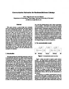
Figure 10: Results for the fth order wave elliptic lter. of lters for both delayed reallocation and immediate reallocation. The algorithms' performances are then compared and contrasted. Our algorithms are coded on a Sparc 10 and run in only seconds for these examples. Figure 10 shows the results for the fth order wave elliptical lter. A few comments should be made to help explain the table. The rst four columns represent the number of CPUs, buses, adders and multipliers respectively, while the AREA column is the total area of these units. The columns under the \Results" heading represent the number of timesteps after variable partition rotation and the total number of interpartition data transfers after variable partition rotation. The columns under the \Needability" heading represent the needability of buses, adders, and multipliers after variable partition rotation is nished. The UNIT column shows which unit type was added based on the needabilities. The area and time constraints may be found at the bottom of the table, as well as the area of the various units and other data. Also note that for this table we did not assume that each software operation took one timestep. Instead, in order to avoid non-integer results, we assumed that software operations took four timesteps while hardware operations took four timesteps. Unless mentioned otherwise, the parameters found in Figure 10 will be used for all other experiments in this section. The elliptic lter in Figure 10 has a critical path of 13. Hence for a software solution the total number of timesteps must be at least 52. Similarly for a hardware solution the total number of timesteps must be at least 39. In order to completely test the system we set the desired time to 39. We know that this solution may only occur when the entire critical path of the system is implemented in hardware. The system begins with 2 CPUs and after list scheduling 80 timesteps are required. 25

At this point the HMS system evaluates which type of hardware is most in demand. It nds that adders are the most in demand; consequently, it adds an adder to the hardware. Variable partition rotation is then used to reschedule the system. This results in a more compact schedule that takes 72 timesteps. Next a multiplier is added to the system. However, by adding a multiplier the area constraint is exceeded. Therefore a CPU is eliminated and list scheduling is again used to obtain a legal schedule. Note that when a CPU is eliminated the number of buses is reset to one. The reason for this is discussed below. After list scheduling is nished, variable partition rotation is again applied, and a new unit of hardware is added based on the resulting needabilities. This process stops when either the time and area constraints have been met, or when the design goals cannot be met with an all hardware implementation. Notice that for the above example the CPU is no longer needed once the time constraint is met. This is probable for this graph since by setting the desired number of timesteps to 39 we assured that the entire critical path of the system needed to be implemented in hardware. Therefore the last row in the gure shows the actual hardware needed once the extra CPU and bus has been eliminated. For most results this extra post processing step would not be necessary; however, if we set the total number of timesteps to very near the hardware minimum some CPUs may not be used. Hence the HMS algorithm checks for this condition and removes these CPUs from the chip. Figure 11 shows the results for a modi ed elliptic lter. The original lter is rst modi ed by multiplying the number of delays on each edge by two (D = Delay Multiplier = 2). Next the lter is unfolded three times. (U = Unfolding Factor = 3). By modifying the input DFGs in this manner a large number of complex lters may be generated from a few simple ones. Also note that in this experiment we continued after the design goals were met until the needability of an all hardware solution was zero for all unit types. Figure 12 shows the results for a larger lter with almost 200 nodes, that has been similarly modi ed. This example runs in less than twenty seconds on a Sparc 10. We will use Figure 11 to analyze the systems performance. It may be seen that as the number of hardware units increases the total interpartition data transfers tends to decrease. For example, for the fourth iteration with 2 CPUs there are over 80 interpartition data transfers; however, for the nal iteration there are less than 40. This pattern is due to the fact that we assume the hardware is to be implemented in a single partition. Hence as more hardware is utilized less buses are needed. In order to oset this eect two things are done. First we reset the number of buses to one whenever a CPU is eliminated. Secondly, after a solution is found we eliminate any buses that have been previously added which are no longer needed. A second trend that may be noted is that when a CPU is eliminated and an equivalent amount of 26

Number of Units CPU BUS ADDERS MULTS AREA 3 1 0 0 165 2 0 0 180 2 1 0 0 115 2 0 0 130 2 1 0 135 3 1 0 150 3 1 1 162 3 2 1 167 3 3 1 172 3 3 2 184 3 4 2 189 1 1 5 2 114 1 5 3 126 1 6 3 131 0 6 3 66

Results TS TT 172 41 124 64 176 41 160 46 144 76 123 82 108 52 93 50 81 24 120 36 108 31 69 11 63 0 63 0 63 0

Area Desired = 190: Time Steps Desired = 63 CPU Area = 50: Bus Area = 15 Hardware Cycles = 3

Needability BUS ADDERS MULTS 2130 1696 64 560 312 64 1400 608 56 300 1304 72 860 448 248 230 272 280 50 424 56 40 376 88 0 144 284 0 168 64 0 96 48 0 16 64 0 16 0 0 0 0

UNIT Bus Bus Bus Adder Bus Mult Adder Adder Mult Adder Adder Mult Adder Mult

Adders Per CPU = 1: Mults Per CPU = 1 Adder Area = 5: Multiplier Area = 12 Software Cycles = 4 Unit = Unit Added TS = Time Steps

TT = Total Interpartition Data Transfers

Figure 11: Results for the elliptic lter with D = 2 and U = 3. hardware is added the number of timesteps may increase. This is due to two factors. First, amount of \equivalent" hardware added when a CPU is eliminated is a conservative estimate. For example, if a CPU contained 8 adders and 10 multipliers and was three times as slow as the hardware being added, we would add 8=3 = 2 adders and 10=3 = 3 multipliers. In the example below, we do not add any hardware since there was only 1 adder and 1 multiplier in the CPU being eliminated. A second reason is that the list scheduling used after a CPU is eliminated may produce a schedule that is not as good as the previous one. It may also be seen that in some cases adding an extra unit of hardware does not decrease the total execution time. For example, when the second multiplier is added to the system after the seventh iteration with two CPUs the number of timesteps increases from 81 to 120. A closer analysis of the complete program output which is not included here due to space considerations reveals that this is due to increased communication time between the new multiplier and the CPUs. This tendency may also be noted by the observation that the number of interpartition data transfers increases from 24 to 36. Figure 13 shows the results for several lters for both delayed reallocation and immediate reallo27

Number of Units CPU BUS ADDERS MULTS AREA 4 1 0 0 215 2 0 0 230 3 1 0 0 165 2 0 0 180 2 1 0 195 3 1 0 150 4 1 0 167 5 1 0 172 5 2 0 184 2 1 0 0 125 2 0 0 140 3 0 0 155 4 0 0 170 5 0 0 185 5 1 0 190 5 2 0 195

Results TS TT 264 71 220 117 276 67 204 100 180 115 192 141 153 147 144 147 140 150 328 89 200 101 184 145 152 153 148 144 144 139 136

Area Desired = 240: Time Steps Desired = 138 CPU Area = 50: Bus Area = 15 Hardware Cycles = 3 TT = Total Interpartition Data Transfers

Needability BUS ADDERS MULTS 6990 5040 128 2860 1272 104 4330 2680 128 2080 1288 112 460 2104 96 2460 688 496 1090 472 280 140 984 424 600 280 432 3910 2304 680 1900 792 472 2480 560 792 1220 400 616 220 856 512 140 696 656

UNIT Bus Bus Bus Bus Adder Bus Bus Adder Bus Bus Bus Bus Bus Adder Adder

Adders Per CPU = 1: Mults Per CPU = 1 Adder Area = 5: Multiplier Area = 12 Software Cycles = 4 Unit = Unit Added TS = Time Steps

Figure 12: Results for the elliptic lter with D = 3 and U = 5. cation. The COMP column is the total number of components is the nal design including adders, multipliers, processors, and global buses. This total is shown since it is a good indicator of how complex the nal design is. It may be noted that the results are the same for all but a few cases. These cases are marked with an asterisk in the lter type column. For the case involving the elliptical lter immediate reallocation takes one extra iteration and requires one extra adder. For the case involving the all-pole lter immediate reallocation takes one fewer iteration and requires one fewer adder. A closer examination of the programs output reveals that while immediate reallocation and delayed reallocation start with dierent initial schedules before variable partition rotation they converge to the same nal schedule after variable partition rotation in nearly all cases. For the few iterations where the two algorithms do not converge to the same nal schedule they often add the same functional unit and converge to the same schedule after the next iteration. While both algorithms produce the same results in the vast majority of cases, our experiences show that immediate reallocation runs in less CPU time than delayed reallocation and is therefore preferred.

28

Filter . Filter Type DM UF Elliptical

* All-Pole

Constraints . AREA TS

1

1

120

2

3

190

4

5

240

1 3

1 4

120 120

5 8 190 * DR = Delayed Reallocation DM = Delay Multiplier TS = Timesteps COMP = Components

Results DR IR IT AREA COMP IT AREA COMP

72 48 110 70 180 136 108

2 5 7 12 4 15 19

24 72 33 88 54

3 4 8 8 17

120 92 162 114 195 195 232

4 6 7 9 6 11 15

2 5 7 12 4 16 19

120 92 162 114 195 200 232

4 6 7 9 6 12 15

87 6 3 87 105 6 4 105 59 6 8 59 185 9 8 185 159 12 16 154 IR = Immediate Reallocation UF = Unfolding Factor IT = Iterations

6 6 6 9 11

Figure 13: Comparison of immediate reallocation and delayed reallocation.

6 Conclusion Hardware/Software co-design is able to create a system rapidly since standardized parts are used to implement most of the system. However, it is also able to meet timing constraints since a limited amount of hardware is used for time critical parts of the system. Important issues in hw/sw co-design include deciding how many hardware components and global buses are needed, partitioning operations between hardware and software, partitioning operations within both the hardware and software domain, and scheduling the hardware after it has been partitioned. In this paper we considered a system which automates the hw/sw co-design process while considering the above factors. There are many design strategies possible in hw/sw co-design. Since design time is often the most important factor, our system attempts to implement as much of the system as possible in software provided that chip area and timing constraints are met. This not only reduces design time but also minimizes test and veri cation time. When considering what hardware to include our system calculates the needability of each type of hardware. The needability of a type of hardware is a measure of how often the system would like to schedule an operation of this type, but cannot due to resource constraints. A similar measure is 29

calculated for global buses. The type of hardware with the greatest needability is added to the system. Once a new unit of hardware is added to the system two algorithms are used to reschedule the system. The rst, delayed reallocation only allows operations to be transferred between partitions during variable partition rotation, a variation of rotation scheduling. The second algorithm, immediate reallocation, transfers groups of operations to the hardware as soon as the hardware is inserted into the system, as well as during variable partition rotation. Results that illustrate the savings which are possible with these algorithms are presented for several data ow graphs.

References [1] S. Antoniazzi, A. Balboni, W. Fornaciari, and D. Sciuto, \HW/SW Codesign for Embedded Telecom Systems," Proceedings of the International Conference on Computer Design, pp. 278-281, Oct. 1994. [2] T. Benner, R. Ernst, I. Koenenkamp, P. Schueler, and H.-C. Schuab, \Prototyping System for Veri cation and Evaluation in Hardware-Software Cosynthesis," Proceedings of the 6th IEEE International Workshop on Rapid System Prototyping, pp. 54-59, 1995. [3] B. Bose, M.E. Tuna, and S.D. Johnson, \Continuations in Hardware-Software Codesign," Proceedings of the International Conference on Computer Design, pp. 264-269, Oct., 1994. [4] B. Bose, M.E. Tuna, and S.D. Johnson, \System Factorization in Codesign: A Case Study of the Use of Formal Techniques to Achieve Hardware-Software Decomposition," Proceedings of the International Conference on Computer Design, pp. 458-461, Oct., 1993. [5] J.P.Calvez,O.Pasqueir, \Performance Assessment of Embedded Hw/Sw Systems," Proceedings of the International Conference on Computer Design, pp. 52-57, Oct. 1995. [6] L.-F. Chao, A. LaPaugh, and E.H.-M. Sha, \Rotation Scheduling: A Loop Pipelining Algorithm," Proc. 30th ACM/IEEE Design Automation Conference, pp. 566-572, June, 1993. [7] P. Chou, R.B. Ortega, and G. Borriello \Interface Co-Synthesis Techniques for Embedded Systems," Proceedings of the International Conference on Computer-Aided Design, pp. 280-287, Nov., 1995. [8] M.R. Garey and D.S. Johnson, \Computers and Intractability - A Guide to the Theory of NP-Completeness". W.H. Freemand and Company, New York, NY, 1979. [9] D. Gaski, F. Vahid, S. Narayan, and J. Gong, \Speci cation and Design of Embedded Systems," Prentice-Hall, Inc, Englewood Clis, NJ, 1994. [10] R. Gupta and G.DeMicheli, \Hardware-Software Cosynthesis for Digital Systems," IEEE Design and Test of Computers, October 1993, pp. 29-41. [11] R. Gupta and G.DeMicheli, \System Level Synthesis Using Re-programable Components," The European Conference on Design Automation, March, 1992 pp. 2-7. [12] J. Henkel, T. Benner, and R. Ernst, \Hardware Generation and Partitioning Eects in the COSYMA System," 2nd International Workshop on Hardware-Software Co-Design, Workshop Handout, 1993. [13] B.K. Holmer and B.M. Prangle, \Hardware/Software Codesign Using Automated Instruction Set Design & Processor Synthesis," Technical Report CS-93-14, Pennsylvania State University, Department of Computer Science, 1993. [14] C.E. Leiserson and J.B. Saxe, \Retiming Synchronous Circuitry," Algorithmica, Vol. 6, 1991, pp. 5-35. [15] M. Sheliga and E. H.-M. Sha, \Bus Minimization and Scheduling of Multi-Chip Modules," The 1995 Great Lakes Symposium on VLSI, Bualo, NY, March, 1995, pp. 40-45.

30

[16] A. Wolfe \A Case Study in Low-Power System-Level Design," Proceedings of the International Conference on Computer-Aided Design, pp. 332-338, Oct., 1995. [17] T.-Y. Yen and W. Wolf \Communication Synthesis for Distributed Embedded Systems," Proceedings of the International Conference on Computer-Aided Design, pp. 288-294, Nov., 1995. [18] T.-Y. Yen and W. Wolf \Performance Estimation for Real-Time Distributed Embedded Systems," Proceedings of the International Conference on Computer Design, pp. 64-694, Oct., 1995.

31