HEAD-RELATED TRANSFER FUNCTION MODELING IN 3-D SOUND SYSTEMS WITH GENETIC ALGORITHMS Ngai-Man Cheung and Steven Trautmann email:
[email protected],
[email protected]
Andrew Horner email:
[email protected]
Texas Instruments Tsukuba R&D Center 17 Miyukigaoka, Tsukuba, Ibaraki 305, Japan
Department of Computer Science Hong Kong University of Science and Technology Clear Water Bay, Hong Kong
ABSTRACT Head-related transfer functions (HRTFs) describe the spectral filtering that occurs between a source sound and the listener's eardrum. Since HRTFs vary as a function of relative source location and subject, practical implementation of 3D audio must take into account a large set of HRTFs for different azimuths and elevations. Previous work has proposed several HRTF models for data reduction. This paper describes our work in applying genetic algorithms to find a set of HRTF basis spectra, and the normal equation method to compute the optimal combination of linear weights to represent the individual HRTFs at different azimuths and elevations. The genetic algorithm selects the basis spectra from the set of original HRTF amplitude responses, using an average relative spectral error as the fitness function. Encouraging results from the experiments suggest that genetic algorithms provide an effective approach to this data reduction problem.
1. INTRODUCTION The purpose of 3-D sound systems is to generate sound fields that appear to emerge from specific elevations and azimuths. To achieve this goal, sound systems simulate auditory cues that humans rely on to determine the positioning of a sound. Among these auditory cues, head-related transfer functions (HRTFs) provide important spatial cues and are widely used in 3-D sound systems. HRTFs describe the spectral filtering that occurs between a source sound and the listener's eardrum. The main filtering elements are the pinnae (the outer ear), and the cavum conchae (the resonant cavity). Previous research on HRTFs has focused on the magnitude component, and the results suggest that HRTF magnitudes vary as a function of frequency, source position, and subject. HRTF magnitudes vary rapidly as a function of frequency, with tremendous peaks and valleys. HRTFs also vary for different source locations horizontally and vertically due to the asymmetric shape of the pinnae. Implementation of 3D audio requires a large set of HRTFs for different azimuths and elevations. Martens [1] and later Wightman and Kistler [2] have investigated a mathematical model to represent HRTFs as a linear combination of a small number of basis spectra. Each particular HRTF magnitude function was expressed as the sum of weighted spectra. HRTF phase was modeled by assuming that HRTFs were minimum phase functions and that inter-aural
phase differences could be approximated by a simple time delay. Wightman and Kistler used five basis spectra to effectively construct 5300 HRTFs, achieving a 30-fold data reduction. The most important step in this model is finding the representative basis spectra. Wightman and Kistler used a statistical approach, principal component analysis (PCA), to compute the basis spectra and weights. One disadvantage of a statistical approach, such as PCA, is that the basis spectra have no physical correlate, but are statistically constructed. This makes the basis spectra potentially difficult to interpret and modify. In this work, we apply genetic algorithms (GAs) to find the basis spectra and normal equation method to find the weights. GAs [3,4] are effective in search and combinatorial optimization problems, using a fitness-directed random search to explore the search space. Section 2 of this paper outlines our genetic algorithm-based HRTF model. Section 3 presents our results, and section 4 concludes the work with suggestions for future work.
2. HRTF MODELING WITH GENETIC ALGORITHMS Figure 1 outlines our procedure for HRTF modeling. We used the KEMAR measurements from MIT [5] as source data. The data set consisted of impulse responses of a dummy head across 710 different positions at elevations from -40 degrees to +90 degrees. Each impulse response was 512 samples long. The measurements included different numbers of equally-spaced azimuths at each elevation. For example, at elevation -40, there were 56 different azimuths sampled every 6.4 degrees. At elevation -30, 60 different azimuths were sampled every 6 degrees. Table 1 lists the number of different azimuths for each elevation. Table 1. Number of Equally-Spaced Azimuths for Each Elevation. Elevation
-40
-30
-20
-10
0
Number of EquallySpaced Azimuths
56
60
72
72
72
50 60 70 80 90 45 36 24 12 1
10 20 30 40 72 72 60 56
directional transfer function (DTF). The set of 710 DTFs are then passed to a GA for selection of representative basis spectra.
Original HRTF Impulse Response FFT Frequency Domain Re-sampling
HRTF Modeling
HRTF Mean Calculation Mean Removal DTF
Encoding Fitness
Mean
Basis Spectra
Genetic Algorithm Optimization
GA Parameters
Reconstructing DTFs requires finding an appropriate set of basis spectra and a weight matrix. Each of the DTFs is represented as a linear combination of basis spectra. If we have the same number of basis spectra as DTFs, then we can reconstruct the DTFs exactly as the original. We only use a few basis spectra in practice to achieve the goal of data reduction. In our experiment, we use only 3 basis spectra to represent the 710 DTFs. The HRTFs can be obtained from the reconstructed DTFs by simply adding back the HRTF mean. The problem can be viewed as the following matrix equation:
AW ≈ B, Weights Matrix
Normal Equation
3-D Positional Control HRTF Re-Construction Matrix Multiplication
Add back Mean
Phase Modeling
(1)
where A is the matrix containing the basis spectra column-bycolumn, W is the weight matrix containing the weights used in the linear combination of the DTFs for different positions, and B is a matrix consisting of DTFs at different positions arranged column-by-column. Expanding equation (1) gives the following equation: a1,1 ... a1, Nbasis a2,1 ... aNfreq,1 ... aNfreq, Nbasis
w1,1 ... w1, NDTF w2,1 × ... wNbasis,1 ... wNbasis, NDTF
b1,1 ... b1, NDTF b2,1 ≈ ... bNfreq,1 ... bNfreq, NDTF
.
(2) Here Nbasis is the number of basis spectra, NDTF is the number of different DTFs at different positions, and Nfreq is the number of frequency points in the DTFs. For our data, NDTF=710 and Nfreq=207. The corresponding system equation is as follows: Nbasis
∑a
(3)
wj , r ≈ bk , r .
k, j
Re-constructed HRTF
Figure 1. HRTF Modeling with Genetic Algorithms. We used the data from the left "normal" pinnae of the MIT dummy head in our experiment. The impulse responses were passed through a 4096-point FFT to obtain the HRTFs. To reduce the data size, we sampled the HRTFs at every semitone (frequency ratio 1:21/12) from 13.75 Hz to 22050 Hz, with the exception of using the frequency ratio 1:21/96 in the range 6000 Hz to 12000 Hz. Many important spectral fluctuations occur in the 10,000 Hz vicinity, which is why we used extra points in that range. The result is 207 frequency points for each HRTF. We tried to obtain samples evenly in each critical band as well as retain the spectral variations of the HRTF. After the FFT and sampling, we calculate and remove the mean function of the HRTFs across all 710 positions from the original HRTFs. The mean HRTF represents the subject-dependent and direction-independent features of the HRTF data set. After removing the mean, each function represents primarily direction-dependent spectral features, and is called the
j =1
In this equation, bk,r is an approximation of the kth frequency point in the rth DTF. Assuming we have found the basis spectra using the GA, we can use the normal equation method [6] to determine the set of weights wj,r which approximate bk,r in the least-squares senses, that is, the wj,r that minimize the squared error:
Nbasis ∑ ak , jwj , r − bk , r ∑ k =1 j =1
Nfreq
2
,
(4)
in the rth DTF. Since each DTF is independent, we can solve for it without consideration of the other DTFs. To determine the basis spectra, we used a genetic algorithm. One possible approach is to let the GA search for the value of each basis spectra frequency point (ak,j). However this is an extremely large search space, and most solutions give bad results. An alternative method is to let the GA select the most
representative DTFs from the original DTF set, and use these representatives as the basis spectra. We assign an index to each DTF, and use the GA to find the indices of the representative DTFs. We encoded the indices into the GA bitstring as shown in Figure 2. Bitstring Length
Table 2. Experiment Parameters for Genetic Algorithm. Number of Basis spectra Total Function Evaluation
…..
S2
S1
to 90 degree range. The GA did not select any basis spectra from the low elevations.
SNbasis
Index Length
2
3
4
5
6
7
8
5000
Population Size
80 120 160 200 240 280 320
Bitstring Length
20 30 40 50 60 70 80
Crossover Rate
0.6
Mutation Rate
0.001
Table 3. Experiment Results Using 3 Basis Spectra. Index Length = ceil ( Log 2
N DTF )
×
Bitstring Length = Index Length
Basis Spectra Selected (Elevation, Azimuth) (40, 84) (50, 320) (80, 180)
N basis
Figure 2. GA Bitstring Encoding. If the GA picks index Sk as one of the basis spectra, and Sk is the DTF at elevation i and azimuth j, then it will be used with the other basis spectra to approximate the DTFs. We use a relative error to measure the quality of reconstructed DTFs compared to the original DTFs. The relative error guides the GA's search for a good solution. The relative error is defined as the following:
1 N ' DTF
N ' DTF
∑ r
∑
N ' freq k
∑
[b
k,r −
N ' freq k
b'k, r]
[bk , r ]2
2
,
(5)
where b'k,r is the rth reconstructed DTF at the kth frequency point. We compare the reconstructed DTF to the corresponding original DTF at N'freq=21 frequency points (one in every ten of the original Nfreq frequencies). This provides a quick estimate of the fitness during the search. Also, only subsets of the original DTFs at azimuths 0, 90, 180, and 270 degrees are used in the relative error calculation. Changes for different azimuths are typically very gradual. This allows the GA to consider each side without taking too much computation, and reduces the number of DTF comparisons to 13 x 4 + 1 = 53.
3. RESULTS We used the GA software package GENESIS Version 5.0 [7] for our experiments, with the parameters listed in Table 2. We performed the experiments on a SUN SPARCstation 5. The turnaround time of the experiment was 10 minutes for 3 basis spectra. Table 3 lists the results for 3 basis spectra. As shown in the table, the three basis spectra are spread evenly at the azimuths 84, 180 and 320 degrees. The results are intuitive since we expect each basis spectrum to represent a different range of azimuths. However, for the elevations, the GA gave some unexpected results. The three basis spectra were all selected from high elevations (40, 50 and 80 degrees) in the original -40
Index 550 633 704
Figure 3 shows some of the reconstructed results. The solid lines show the original HRTFs and the dotted lines show the reconstructed HRTFs. The HRTFs of Figure 3-1 are from elevation -40, azimuth 186. This location is far away from any of the basis spectra. As shown in the figures, our method gives a very close approximation to the original, although there are some small differences in the spectral regions with lots of peaks and valleys. Figure 3-2 shows a comparison at elevation -30, azimuth 336. This location has the worst relative error between the original and re-constructed HRTF. As shown in Figure 3-2, there are several larger deviations between the original and reconstructed functions in the spectral regions from 6kHz to 11kHz. However, overall the reconstructed function basically matches the original. We have performed experiments using 5 basis spectra, and Table 4 shows the results. In this case the GA selected basis spectra from low elevations (-20, -10) as well. This improved the re-construction of low-elevation HRTFs. Table 4. Experiment Results Using 5 Basis Spectra. Basis Spectra Selected (Elevation, Azimuth) (-20, 5) (-10, 130) (-10, 180) (40, 96) (70, 285)
Index 118 215 225 552 693
Figure 4 shows the relative errors and data reduction plotted against number of basis spectra. Data reduction is given by the amount of original data over the amount of reconstructed data. As expected by using more basis spectra we achieve better relative error but less data reduction. Also, using more than 3
of the spectral variations of the originals, while achieving a 50fold data reduction. 90
0.05
80 Data Reduction
0.045
Relative Error
60
0.04
50 0.035 40
30
Average Relative Error
Data Reduction (Original / GA Modeling)
70
0.03
20 0.025 10
Figure 3-1. Elev:-40 Azim: 186
0
0.02 0
1
2
3
4
5
6
7
8
9
No of Basis Spectra Using
Figure 4. Relative Errors and Data Reduction plotted against Number of Basis Spectra. There are several related research topics. We might improve the results by designing a better fitness function in the GA optimization. For example, we can incorporate our prior knowledge about the typical shape of HRTFs into the fitness function. Moreover, we can expand our data set to include measurements from more subjects and locations. With the symmetry of GAs, we can easily parallelize the system to handle large data sets.
5. REFERENCES
Figure 3-2. Elev:-30 Azim: 336
Figure 3. Comparisons between the Original HRTFs (Solid Lines) and the Reconstructed HRTFs (Dotted Lines).
basis spectra gives a smaller improvement in relative error for an additional basis spectra.
4. SUMMARY We have introduced the use of genetic algorithms to HRTF modeling. The GA determines the basis spectra and normal equation method determines the weights. We have implemented and tested the method. Empirical results show that with only 3 basis spectra we were able to reconstruct HRTFs closely resembling the original HRTFs, including most
[1] Martens, W., "Principal components analysis and resynthesis of spectral cues to perceived direction," in Proceedings of the International Computer Music Conference, International Computer Music Association, San Francisco, CA, 274-281, 1987. [2] Kistler, D., and Wightman, F., "A model of head-related transfer functions based on principal components analysis and minimum-phase reconstruction," Journal of the Acoustical Society of America, 91, 1637-1647. [3] Goldberg, D. E., Genetic Algorithms in Search, Optimization, and Machine Learning. Addison-Wesley Publishing Company, Inc., 1989. [4] Cheung, N.-M., and Horner, A. B., "Group synthesis with genetic algorithms," Journal of the Audio Engineering Society, vol.44, no.3 (March 1996), 130-47. [5] Gardner, B., and Martin, K., "HRTF Measurements of a KEMAR Dummy-Head Microphone," MIT Media Lab Technical Report #280, May 1994. [6] Kahaner, D., Moler, C., and Nash, S., Numerical Methods and Software. Prentice Hall, 1989. [7] Grefenstette, J. J., A Users Guide to GENESIS, Version 5.0, October 1990.