distribute the vertices of the triangle mesh over the iso-surface and generate a triangle mesh ..... Proceedings, pages 389â396, 2000. [3] A. Certain, J. Popovic, ...
Hierarchical Iso-Surface Extraction Ulf Labsik
Kai Hormann
Martin Meister
G¨unther Greiner
Computer Graphics Group University of Erlangen
Multi-Res Modeling Group Caltech
Computer Graphics Group University of Erlangen
Computer Graphics Group University of Erlangen
Figure 1: First three levels and final result of our hierarchical iso-surface extraction algorithm.
Abstract The extraction and display of iso-surfaces is a standard method for the visualization of volume data sets. In this paper we present a novel approach that utilizes a hierarchy on both the input and the output data. For the generation of a coarse base mesh, we construct a hierarchy of volumes and extract an iso-surface from the coarsest resolution with a standard Marching Cubes algorithm. We additionally apply a simple mesh decimation algorithm to improve the shape of the triangles. We iteratively fit this mesh to the iso-surface at the finer volume levels. To be able to reconstruct fine detail of the iso-surface we thereby adaptively subdivide the mesh. To evenly distribute the vertices of the triangle mesh over the iso-surface and generate a triangle mesh with evenly shaped triangles, we have integrated a mesh smoothing algorithm into the fitting process. The advantage of this approach is that it generates a mesh with subdivision connectivity which can be utilized by several multiresolution algorithms such as compression and progressive transmission. As applications of our method we show how to reconstruct the surface of archaeological artifacts and the reconstruction of the brain surface for the simulation of the brain shift phenomenon.
1
Introduction
Rendering iso-surfaces is a standard technique in scientific visualization of volume data and the Marching Cubes algorithm (MC) [16] is commonly used for constructing iso-surfaces which are represented as triangle meshes. The main drawback of this method is that it produces meshes with many small and badly shaped triangles. Such meshes require improvement with decimation, smoothing, or remeshing. These post processing algorithms can be very expensive in terms of time and memory consumption, especially if the meshes are large. And with the resolution of today’s scanning devices, the output mesh of MC can easily consist of millions of triangles. We therefore propose to down-scale the volume data set and create a hierarchy of volumes as described in Section 3. Then we use MC to extract the iso-surface on the coarsest resolution and fit the mesh to the iso-surfaces at the finer levels of the volume hierarchy
later. Since the number of triangles in the extracted mesh depends quadratically on the resolution of the volume, performing MC on the coarsest level yields a mesh with low complexity which can be optimized efficiently. We apply a strategy for improving the MC mesh by removing short edges so as to obtain a base mesh with few and well-shaped triangles. Once this base mesh is constructed, we use it as an initial guess for approximating the iso-surface on the next finer volume level and iterate this fitting process until we arrive at an iso-surface reconstruction with respect to the original data. Our fitting procedure is discussed in Section 4 and takes three aspects into account. Firstly, the vertices of the mesh need to be projected onto the iso-surface as we want to sample that surface. Secondly, a relaxation operator is required to evenly distribute the sample points over the surface and to ensure well-shaped triangles in the final mesh. Thirdly, we adaptively subdivide the mesh in order to approximate the iso-surface within a user-specified accuracy and to capture local detail. In this way we finally obtain a semi-regular mesh with a hierarchical structure that can be utilized by many multiresolution algorithms such as level-of-detail rendering [3], progressive transmission [10, 14], multiresolution editing [31], and wavelet decomposition and reconstruction [17, 22]. As an application of the method we have reconstructed the surfaces of archaeological artifacts like the one in Figure 1 from CT scans as well as a human brain from an MRI scan. We present the results in Section 5 and conclude in Section 6.
2
Related Work
The standard approach for the extraction of iso-surfaces from volume data is the well known Marching Cubes (MC) algorithm [16]. The algorithm walks through all cells of a regular hexahedral grid and computes the iso-surface for each cell independently. In order to avoid ambiguities of MC, several modifications were proposed [19, 20] and an extension to reconstruct surfaces with sharp features from distances volumes was presented by Kobbelt et al. [13]. To improve the performance of MC, several algorithms [6, 27, 29] use adaptive hierarchies of the volume data set.
(a)
(b)
(c)
(d)
Figure 2: Iso-surface M 2 (900) using box filter (a), Gauß filter (b), median filter (c), and dilation (d) to compute f 2 .
The task of converting an arbitrarily triangulated mesh into a semi-regular mesh is called remeshing. In the approach of Eck et al. [5], vertices are distributed over the given triangulation and a base mesh is constructed by growing geodesic Voronoi tiles around the vertices. A parameterization of the given triangulation within the base triangles is computed by using harmonic maps which minimize the local distortion. The remesh is then determined by uniformly subdividing each base triangle and mapping the vertices into 3-space using the parameterization. Lee et al. [15] construct the base mesh by mesh reduction based on edge collapses and incrementally compute a parameterization of the original triangulation within the triangles of the remaining mesh. This process leads to a locally smooth parameterization. In order to achieve a global smoothness the dyadic points are moved by a variant of Loop’s subdivision scheme and mapped into 3-space. Kobbelt et al. [12] describe a shrink-wrapping approach for remeshing. The idea is to place a semi-regular mesh around the original surface. Analogously to the physical shrink-wrapping by exhausting the air between both surfaces the semi-regular mesh is shrunk onto the surface. In addition, a relaxation force is used to distribute the vertices uniformly over the surface. The direct extraction of semi-regular meshes from volume data is addressed by several papers. Bertram et al. [2] use MC to extract an initial iso-surface which is coarsened by a mesh simplification algorithm based on [7]. Then they use a modified shrinkwrapping approach to compute their final semi-regular mesh based on a quadrilateral subdivision scheme. A method for directly extracting a coarse base mesh from the volume was presented by Wood et al. [30]. They compute contours of the surface from the volume data and connect them such that they form a coarse mesh which is topologically equivalent to the desired iso-surface. The final semi-regular mesh is constructed by using a multi-scale forcebased solver with an external force moving the vertices to the isosurface and an internal force relaxing the vertices of the mesh.
3
sions nx , ny , and nz , G0 = {(xi , yj , zk ) : 0 ≤ i ≤ nx , 0 ≤ j ≤ ny , 0 ≤ k ≤ nz }, (1) with xi = x0 + i hx , yj = y0 + j hy , zk = z0 + k hz . In order to simplify notation, we further assume a consistent grid size h = hx = hy = hz . A hierarchy f 0 , f 1 , f 2 , . . . , where each f l is defined on a grid Gl with grid size 2l h and dimensions �2−l nx �, �2−l ny �,�2−l nz �, can then be computed by iteratively down-sampling the volume data by a factor of two. This process is usually realized by convolving the function fl−1 with a suitable filter and then sampling the filtered signal to obtain f l . We assume that the gray values of the object we want to reconstruct are larger than the gray values of the surrounding voxels. We have tested several filters, including box, Gauß and median filter, but found the dilation operator to perform best within the scope of our investigations, as illustrated in Figure 2. This operator selects the largest gray value from the cluster of eight voxels on level l−1 that are combined to form the corresponding voxel with double edge length on level l and defines f l (xi , yj , zk ) =
max
i� ∈{i,i+1} j � ∈{j,j+1} k� ∈{k,k+1}
f l−1 (xi� , yj � , zk� ),
(2)
where i, j, and k are multiples of 2l . Given an iso-value v, we can now extract an approximation M l (v) of the corresponding isosurface from the down-sampled data set f l with a standard marching cubes algorithm [16]. Figure 3 shows that the use of low-pass filters tends to wash out thin voxel layers which represent the object’s material. This may result in topological holes as illustrated in Figures 2 (a)-(c). In contrast, the dilation operator has a growing effect and for a fixed iso-value, M l can in fact be proven to encompass the meshes
Base Mesh Construction v
In order to efficiently create a base mesh with few triangles, we run a marching cubes algorithm on a coarse volume which is computed by down-sampling the given data. As the number of triangles generated by marching cubes depends quadratically on the number of voxels in each dimension, scaling down the volume by a factor of n reduces the complexity of the extracted mesh by n2 . Suppose the volume data to be represented as a discrete gray value function f 0 : G0 → IN, defined on a regular grid of dimen-
(a)
(b)
(c)
Figure 3: Filtering the input signal: (a) original voxels, (b) voxels after low-pass filtering, (c) voxels after dilation.
4
Iso-Surface Fitting
Due to the growing effect of the dilation operator, the vertices of the base mesh do not lie on the iso-surface at level 0 that we actually want to reconstruct, and we have to shrink the mesh onto that surface. In order to increase robustness and performance of that algorithm, we utilize the previously constructed hierarchy of volumes by iteratively fitting the mesh to the next finer level. We first move the vertices to the iso-surface at level l − 1, then to the one at level l − 2, and so on, until we finally arrive at level 0. Note that this always guarantees the vertices of the current mesh to be close to the iso-surface, namely within distance of 2 voxels. This helps to avoid self-intersections of the triangulation after projecting the vertices which may occur if the distance is too large as mentioned in [12]. The essential step of our hierarchical iso-surface extraction algorithm is to adaptively fit the current mesh to the iso-surface of the volume at a certain level l. Such an iso-surface Sl (v) is defined as Figure 4: Iso-surfaces M 3 (900) (gray) and M 0 (900) (green). M l−1 , M l−2 , . . . , M 0 extracted from the finer levels as illustrated in Figure 4. Although this method may modify the topology of the iso-surface, as small holes can vanish as a result of the dilation in general, it is appropriate for the data sets we consider because they are topologically simple. A typical phenomenon of the marching cubes algorithm is that some of the generated triangles are very small. In fact, whenever the difference δ of a voxel’s gray value to the specified iso-value v is small, the algorithm cuts off a corner of the underlying grid and creates a triangle whose size is proportional to δ. Due to their tininess it is reasonable to assume that these triangles do not contain significant geometrical information. As we finally aim to generate a triangulated iso-surface with evenly distributed vertices, we perform a decimation step before further processing the mesh. In order to remove all edges that are shorter than a certain threshold length α2l h with α > 0, we first replace all the triangles with three short edges by a single vertex at their barycenter (see Figure 5 (a)) and then collapse the remaining short edges to their midpoints (see Figure 5 (b)). We found that α = 0.5 is a good choice and this simple strategy reduces the number of triangles by approximately 20%.
(a)
(b)
Figure 5: Removing short edges from the extracted iso-surface with a two-pass mesh decimation algorithm.
S l (v) = {(x, y, z) : f˜l (x, y, z) = v}
(3)
where f˜l : [Gl ] → IR is the continuous extension of f l which trilinearly interpolates the values f l (Gl ). The three ingredients of this fitting procedure which are repeated iteratively are the following: 1. Moving the vertices to the iso-surface (projection). 2. Improving the distribution of the vertices (relaxation). 3. Adaptively subdividing the mesh (refinement).
4.1 Projection As the iso-surfaces S l+1 and S l are different, the vertices of the current mesh will not lie on S l and we need a method for projecting them onto that surface. In principle, this can be done by finding the first intersection of a ray emanating from that vertex in a certain direction with S l , but the question remains how to determine the direction of that ray. We could, for example, use the gradient of the gray value function f 0 , as it is often done in volume rendering [11, 21, 28]. While this choice works well in medical applications, we found it inappropriate for our kind of data for the following reason. The objects that we wish to reconstruct are made of a rather homogeneous material. If the volume data had an infinitesimal resolution, it would ideally be a binary data set with gray value zero in those voxels which represent the air surrounding the object and a material-dependent constant gray value in all other voxels. Therefore the gradient of the gray value function is either zero or undefined. In practice, this proposition does not hold because any scanning device has finite resolution only and is susceptible to measuring errors. However, we found the gray value gradient to be too noisy for our purposes. Another choice is the gradient of the distance function dl : l [G ] → IR which gives the shortest signed distance of a point to the iso-surface S l [8, 9]. For volumes, such a distance function is usually defined by the values at the grid points Gl and trilinear interpolation, just as f˜l , and the values at the grid points are determined by a fast marching method [23]. The distance gradient proved to be a better choice than the gray value gradient but it also has some potential drawbacks. Firstly, it is not properly defined everywhere, because it is discontinuous along the medial axis of Sl , and thus the evaluation of the gradient is extremely unstable near the medial axis. However, since the current mesh is guaranteed to be close to S l this is not an issue for our computations, but a more serious drawback is that the distance gradient is not capable of moving vertices inside a concave region of the iso-surface as illustrated in Figure 6.
nv
regions where the object is also very thin so that the two parts of the iso-surface are close. In this case we consider the ray along the positive normal direction and find the first (c) or second (d) intersection with the iso-surface. In order to distinguish between the cases (a,b) and (c,d) we determine the sign of the scalar product < nv |gv >. Although the distance gradient is not defined on the medial axis no problems will occur, because in both cases (b) and (c) the vertex will be moved along the positive normal direction. To check if the correct intersection was found in case (d) we again use the sign of the scalar product < nv |gv >.
nv
gv gv
Sl
4.2 Relaxation Figure 6: Iso-surface S l with iso-distance lines (dotted) and distance gradients gv and normals nv at two vertices of the mesh.
A problem of this projection method is that it may lead to a local clustering of vertices or even self-intersections of the triangulation. By additionally applying a relaxing force we can overcome this drawback and ensure an even distribution of the vertices over the iso-surface. A common approach is to apply a discrete version of the Laplacian, L(v) =
1 � (w − v), |Nv |
(5)
w∈Nv
(a)
as it was done, for example, in [24, 4, 12] in order to smooth or denoise meshes. But this operator has a shrinking effect on the mesh and moves vertices far off the iso-surface in highly curved regions. We therefore follow the strategy in [30] and use only the tangential part of the Laplacian,
(b)
T (v) = L(v)− < L(v)|nv > nv ,
(6)
for smoothing the parameterization of the mesh and keeping the vertices close to the iso-surface. (c)
(d)
4.3 Refinement Figure 7: Distance gradient and normal vector at a vertex in four different situations. The gray-shaded region indicates the region enclosed by the iso-surface and the dashed line its medial axis. We therefore move the vertex v along the direction of the normal vector nv at v which can either be found by averaging the normals of the triangles adjacent to v or, as we did, by normalizing the curvature normal vector [4]
�(v) =
�
(cot αw + cot βw )(v − w),
(4)
w∈Nv
where Nv is the set of v’s neighboring vertices and αw and βw are the angles opposite to the edge vw in the adjacent triangles. Once the normal is computed, we need to evaluate whether the intersection with the iso-surface can be found in the positive or negative direction. Figure 7 shows the different cases that can occur and we use the distance function and its gradient to recognize them. Normally, the vertex is near the iso-surface and we can simply use the sign of the distance function to decide on which side of the surface it lies on. If dl (v) > 0 then the vertex lies ‘outside’ and we move it into the opposite direction of its normal vector (a). If dl (v) < 0 then it is located ‘inside’ and needs to be pushed along the normal direction (b). Both cases have in common that the normal vector nv and the distance gradient gv point in opposite directions. It may also happen that nv and gv are oriented similarly as in (c) and (d), indicating that the vertex is beyond the medial axis and close to the ‘wrong’ iso-surface. This can happen if the refinement step insert new vertices into the mesh at highly curved
In order to approximate the iso-surface within a user-specified accuracy and to capture local detail we adaptively subdivide a triangle of the mesh depending on a refinement criterion. For a triangle T = [u, v, w] we evaluate the distance function at a number of sample points αu + βv + γw with α + β + γ = 1, and quadrisect the triangle if at least one of these vertices is further from the iso-surface than a given ε. After subdividing a triangle, the newly inserted vertices are projected onto the iso-surface as described in Section 4.1. There are a few restrictions in this adaptive subdivision approach. As we want to keep the number of special configurations small we only allow balanced meshes, i.e. the refinement level of two neighboring triangles may only differ by one and we use the special technique of red-green triangulations [1, 25, 26] to avoid cracks in the mesh where two triangles from different levels meet.
5
Results
In cooperation with the Archaeological Institute and the Neuroradiology Center at the University of Erlangen, we have scanned archaeological artifacts with a medical CT scanner and used our algorithm to reconstruct the surfaces. The leftmost picture in Figure 1 shows the base mesh as extracted from the coarsest volume after decimation. In the middle, the meshes are shown after fitting them to the iso-surfaces of the next finer volume levels. In both steps a uniform subdivision step was performed. The rightmost picture shows the final result after two further adaptive subdivision steps which was fitted to the iso-surface at the finest volume resolution and smoothed within the user-specified tolerance.
iso-surface from the original volume data set, and coarsen it by a mesh reduction algorithm. In contrast to our approach this would be much more time and memory consuming. The volume hierarchy also increases the robustness of our algorithm, since the extracted surface can be fitted iteratively to finer levels of the volume until the original resolution is reached. A potential drawback of our method is that the dilation operator may change the topology of the iso-surface as small holes can disappear. Therefore, the presented algorithm may fail to generate topologically correct iso-surfaces for more complex volume data sets, like the results from numerical simulations or medical data sets, where the topology of an iso-surface must not be changed. This issue was not a problem for the data sets we considered, since they were topologically simple. However, it remains a problem to be addressed in future work.
Acknowledgments Figure 8: Examples of vertical sections from the reconstructed surfaces in Figures 1 and 9.
As can be seen from the vertical section of that mesh in Figure 8, we did not only reconstruct the outer but also the inner surface of this item which appears to be hollow. Such cross-sections are of vital importance since they allow the archaeologist to study the profile and the wall thickness of the object which helps to identify the period in which they were crafted or even the specific potter. The other section in Figure 8 was taken from the surface in Figure 9 and a final example is illustrated in Figure 10. Although algorithm was originally designed to handle this kind of objects, we found it appropriate for other purposes as well. Figure 11 shows the reconstruction of a human brain from an MRI scan, which was later used for the simulation of the brain shift phenomenon [18]. The data set was segmented with the help of a semiautomatic algorithm to separate the brain volume from the rest of the data set. Table 1 lists the size of the volumes from that were used in the examples and the number of hierarchy levels used. It also summarizes the information about the extracted iso-surface and the approximation error with respect to a mesh produced using marching cubes on the full resolution of the volume data set. The performance of the algorithm was measured on an AMD Athlon with 1.2 GHz.
6
Conclusion
In this paper we presented a new approach for hierarchically extracting iso-surfaces as semi-regular meshes from volume data. The main purpose of this algorithm is the reconstruction of objects scanned by a CT or MRI scanner, like Archaeological items or the brain surface as presented in the previous section. Our method utilizes a multiresolution representation of the given volume. The hierarchy levels are computed by filtering the volume with a dilation filter and subsampling it afterwards. A coarse base mesh is created by extracting and then simplifying the iso-surface from the coarsest resolution. The iso-surfaces on the finer volume levels are iteratively captured by a fitting procedure that not only projects the vertices of the current mesh onto the iso-surface but also takes care of the vertex distribution and adaptively refines the mesh to approximate local detail. Our method was inspired by the shrink-wrapping approach for remeshing arbitrarily connected triangle meshes [12] but the hierarchical setting improves robustness and performance of that algorithm. Using a coarsened volume accelerates the generation of a coarse base mesh. The alternative approach would be to extract an
We would like to thank Dr. Martin Boss from the Archaeological Institute from the University of Erlangen-Nuremberg for providing the archaeological items and Dr. Bernd Tomandl from the Neuroradiology for scanning the objects.
References [1] R. E. Bank, A. H. Sherman, and A. Weiser. Refinement algorithms and data structures for regular local mesh refinement. In R. Stepleman, editor, Scientific Computing, pages 3–17, Amsterdam, 1983. IMACS/North Holland. [2] M. Bertram, M. A. Duchaineau, B. Hamann, and K. I. Joy. Bicubic subdivision-surface wavelets for large-scale isosurface representation and visualization. In Visualization 2000 Proceedings, pages 389–396, 2000. [3] A. Certain, J. Popovi´c, T. DeRose, T. Duchamp, D. Salesin, and W. Stuetzle. Interactive multiresolution surface viewing. In ACM Computer Graphics (SIGGRAPH ’96 Proceedings), pages 91–98, 1996. [4] M. Desbrun, M. Meyer, P. Schr¨oder, and A. H. Barr. Implicit fairing of irregular meshes using diffusion and curvature flow. In ACM Computer Graphics (SIGGRAPH ’99 Proceedings), pages 317–324, 1999. [5] M. Eck, T. DeRose, T. Duchamp, H. Hoppe, M. Lounsbery, and W. Stuetzle. Multiresolution analysis of arbitrary meshes. In ACM Computer Graphics (SIGGRAPH ’95 Proceedings), pages 173–182, 1995. [6] T. Gerstner and R. Pajarola. Topology preserving and controlled topology simplifying multiresolution isosurface extraction. In IEEE Visualization 2000, pages 259–266, 2000. [7] H. Hoppe. Progressive meshes. In ACM Computer Graphics (SIGGRAPH ’96 Proceedings), pages 99–108, 1996. [8] H. Hoppe, T. DeRose, T. Duchamp, M. Halstead, H. Jin, J. McDonald, J. Schweitzer, and W. Stuetzle. Piecewise smooth surface reconstruction. In ACM Computer Graphics (SIGGRAPH ’94 Proceedings), pages 295–302, 1994. [9] H. Hoppe, T. DeRose, T. Duchamp, J. McDonald, and W. Stuetzle. Mesh optimization. In ACM Computer Graphics (SIGGRAPH ’93 Proceedings), pages 19–26, 1993. [10] A. Khodakovsky, W. Sweldens, and P. Schr¨oder. Progressive geometry compression. In ACM Computer Graphics (SIGGRAPH ’00 Proceedings), pages 271–278, 2000.
Figure 9: Original and reconstruction of a drinking pot featuring a pygmy (Athens, 5th century b.c.).
Figure 10: Original and reconstruction of a red-figured amphora (Athens, 5th century b.c).
Figure 11: Adaptive reconstruction of the brain surface from a segmented MRI data set. name
volume
isis amphora pygmy brain
256x256x128 256x256x256 256x144x256 256x256x112
hierarchy levels 4 5 4 5
triangles (base) 2225 1397 1478 198
triangles (final) 142400 89408 119292 70630
hierarchy levels 4 4 ≤5 ≤5
triangles (MC) 284606 932166 383524 258316
approx. error 0.032% 0.018% 0.036% 0.12%
time/s 16.05 79.02 87.5 118
Table 1: Size, approximation error and reconstruction time of the presented models.
[11] J. Kniss, G. Kindlmann, and C. Hansen. Interactive volume rendering using multi-dimensional transfer functions and direct manipulation widgets. In Visualization 2001 Proceedings, 2001. [12] L. Kobbelt, J. Vorsatz, U. Labsik, and H.-P. Seidel. A shrink wrapping approach to remeshing polygonal surfaces. In Computer Graphics Forum (EUROGRAPHICS ’99 Proceedings), volume 18, pages 119–130, 1999. [13] L. P. Kobbelt, M. Botsch, U. Schwanecke, and H.-P. Seidel. Feature sensitive surface extraction from volume data. In ACM Computer Graphics (SIGGRAPH ’01 Proceedings), pages 57–66, 2001. [14] U. Labsik, L. Kobbelt, R. Schneider, and H.-P. Seidel. Progressive transmission of subdivision surfaces. Computational Geometry, 15:25–39, 2000. [15] A. W. F. Lee, W. Sweldens, P. Schr¨oder, L. Cowsar, and D. Dobkin. MAPS: Multiresolution adaptive parameterization of surfaces. In ACM Computer Graphics (SIGGRAPH ’98 Proceedings), pages 95–104, 1998. [16] W. E. Lorensen and H. E. Cline. Marching cubes: A high resolution 3D surface construction algorithm. In ACM Computer Graphics (SIGGRAPH ’87 Proceedings), pages 163– 169, 1987. [17] M. Lounsbery, T. DeRose, and J. Warren. Multiresolution analysis for surfaces of arbitrary topological type. ACM Transactions on Graphics, 16:34–73, 1997. [18] M. Miga, K. Paulsen, P. Hoopes, F. Kennedy, and A. Hartov. In vivo analysis and modeling of interstitial pressure in the brain under surgical loading. J. Biomech. Eng., 122(4):354– 363, 2000.
[21] C. Rezk-Salama, K. Engel, M. Bauer, G. Greiner, and T. Ertl. Interactive volume rendering on standard PC graphics hardware using multi-textures and multi-stage rasterization. In Proc. SIGGRAPH/Eurographics Workshop on Graphics Hardware, 2000. [22] P. Schr¨oder and W. Sweldens. Spherical wavelets: Efficiently representing functions on the sphere. In ACM Computer Graphics (SIGGRAPH ’95 Proceedings), pages 161– 172, 1995. [23] J. Sethian. Level Set Methods and Fast Marching Methods. Cambridge University Press, UK, 1999. [24] G. Taubin. A signal processing approach to fair surface design. In ACM Computer Graphics (SIGGRAPH ’95 Proceedings), pages 351–358, 1995. [25] M. Vasilescu and D. Terzopoulus. Adaptive meshes and shells: Irregular triangulation, discontinuities, and hierarchical subdivision. In Proceedings of Computer Vision and Pattern Recognition conference, pages 829–832, 1992. [26] R. Verf¨urth. A review of a posteriori error estimation and adaptive mesh refinement techniques. Wiley-Teubner, 1996. [27] G. Weber, O. Kreylos, T. Ligocki, H. Hagen, B. Hamann, and K. Joy. Extraction of crack-free isosurfaces from adaptive mesh refinement data. In Proceedings of VisSym 2001, pages 25–34, 2001. [28] R. Westermann and T. Ertl. Efficiently using graphics hardware in volume rendering applications. In ACM Computer Graphics (SIGGRAPH ’98 Proceedings), pages 169–179, 1998. [29] R. Westermann, L. Kobbelt, and T. Ertl. Real-time exploration of regular volume data by adaptive reconstruction of isosurfaces. The Visual Computer, (2):100–111, 1999.
[19] C. Montani, R. Scateni, and R. Scopigno. A modified lookup table for implicit disambiguation of marching cubes. The Visual Computer, 10:353–355, 1994.
[30] Z. Wood, M. Desbrun, P. Schr¨oder, and D. Breen. Semiregular mesh extraction from volumes. In Visualization 2000 Proceedings, pages 275–282, 2000.
[20] G. Nielson and B. Hamann. The asymptotic decider: resolving the ambiguity in marching cubes. In Visualization 1991 Proceedings, pages 83–91, 1991.
[31] D. Zorin, P. Schr¨oder, and W. Sweldens. Interactive multiresolution mesh editing. In ACM Computer Graphics (SIGGRAPH ’97 Proceedings), pages 259–268, 1997.