Wavelets in Computer Graphics - Caltech Multi-Res Modeling Group

1

Wavelets in Computer Graphics Peter Schr¨oder California Institute of Technology Abstract One of the perennial goals in computer graphics is realism in realtime. Handling geometrically complex scenes and physically faithful descriptions of their appearance and behavior, clashes with the requirement of multiple frame per second update rates. It is no surprise then that hierarchical modeling and simulation have already enjoyed a long history in computer graphics. Most recently these ideas have received a significant boost as wavelet based algorithms have entered many areas in computer graphics. We give an overview of some of the areas in which wavelets have already had an impact on the state of the art. Keywords Computer graphics, wavelets, rendering, curves, surfaces, volumetric data, compression, analysis, variational modeling, interactive modeling, second generation wavelets.

I. I NTRODUCTION Research in computer graphics (CG) has recently seen considerable activity centered around the use of wavelets. As in many other disciplines, the ideas of multiple levels of resolution, or so called “level of detail” modeling, have been around in CG for a long time. Thus when wavelets moved from a mathematical analysis tool to a practical computational tool they were quickly put to use in CG. There are several reasons for the enthusiastic welcome wavelet based algorithms have received in CG. Foremost stand the huge computational demands of CG applications. Geometric models, for example, are often built from a large number of primitive elements in order to achieve some desired level of fidelity with respect to a real world object. At the same time users want all manipulations and computations involving these objects to occur interactively, i.e., with screen updates occurring multiple times per second. Similarly, shading and motion of these objects should appear realistic. Depending on the number and complexity of objects occurring in the scene this can lead to very expensive algorithms. Examples include the modeling of constrained dynamical systems, deformation of objects under forces, and indirect illumination effects. Performing the necessary computations under the constraints of interactivity demands the most efficient algorithms possible, and shrewd approximations without sacrificing perceived realism. Due to the ability of wavelets to represent functions and datasets compactly within user specified error bounds they are a natural tool to consider. Their “zooming in” ability allows the use of “just enough” precision in a given region of interest while at the same time allowing coarse representations in regions outside the immediate area of interest. Even more importantly, they facilitate a smooth tradeoff between computation time, and resulting simulation quality. Often the algorithms which manipulate these hierarchical objects become asymptotically faster as well, allowing the use of much larger and more complicated scenes than previously possible. In this paper we to give a brief overview of the many applications in CG to which wavelets have already made a contribution. Since the areas are numerous we favor breadth over depth at times and refer the interested reader to the original papers and the references therein for more details. We begin with a more in depth description of the use of wavelets in illumination computations, since there has been considerable activity in that area in particular. This is followed by a review of the use of wavelets in modeling curves, surfaces, and animation paths, their extension to more general domains, and scientific visualization and processing of 3D data sets. II. I LLUMINATION C OMPUTATIONS Computing the illumination in a virtual scene is one of the basic problems of CG. It can be computed at many different levels of fidelity. At the high speed but low quality end, we find graphics workstation hardware capable of shading more than 1 million polygons per second with simple local illumination models. On the other hand, algorithms which are capable of capturing the subtle gradations due to indirect illumination and area light sources require considerably larger resources. High fidelity images based on a whole range of reflection phenomena described by the rendering equation [32] often take hours or days to compute. The high complexity of such computations is a consequence of the fact that each surface in a scene can potentially affect the appearance of every other surface, leading to very large and dense linear systems. One algorithm known as radiosity [13] makes the simplifying assumption that all reflection in an environment occurs diffusely to reduce the general case to a manageable, albeit still very expensive, simulation. Diffuse reflection is a reasonable assumption for such interior surfaces as matte walls, but more problematic for polished wood, for example. In spite of this limitation, algorithms that compute radiosity solutions, for example in architectural environments, have been very popular, and in this particular area wavelets have had a large impact.

2

E x

θx

R

E E

I

r R

θy

I

R y Box (nodal) basis

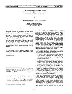
Fig. 1. On the left the geometry for the interaction between point x and y on some pair of surfaces. On the right a simple environment in “flatland,” two parallel line segments and the resulting matrix of couplings using 32 constant elements (adapted from [49]).

Radiosity, B(y), with units [W /m2 ], is a function defined over all surfaces M2 ⊂ R3 which make up a given scene. It is governed by a Fredholm integral equation of the second kind B(y) = Be (y) + ρ(y)

Z

M

2

G(x, y)B(x) dx with G(x, y) =

cosθx cos θy V (x, y), 2 π rxy

(1)

which states that radiosity at surface point y is the sum of an emitted part, Be (y), and a reflection term due to radiosities on all other surfaces. The fraction of light reflected is given by ρ, and the irradiance by an integral over all other surfaces in which the radiosity is weighted by a geometry term G(x, y). It accounts for relative orientation through the cosines of the local surface normals with −2 , with distance, and a visibility function V , which takes on the values 1 and 0 if x can the line connecting x and y, the falloff, rxy or cannot “see” y respectively (see Figure 1, left). To simplify the exposition we will assume that the world is monochrome. In practice Equation 1 is typically solved for 3 representative wavelengths, (r, g, b). A common approach to solve such integral equations is the use of finite elements. Classically [22], [46] constant elements have been used in CG. The scene is meshed into many small surfaces, each with a constant radiosity, resulting in a discrete approximation of Equation 1 Z Z ∀i : bi = bei + ρi ∑ Gi j b j where Gi j =

G(x, y)N j (x)Ni (y) dx dy.

(2)

j

This linear system is characterized by coupling coefficients Gi j . The solution to this system is a set of coefficients bi of an approximation Bˆ = ∑i bi Ni to the actual solution B, where {Ni }i=1,...,n is the basis corresponding to the elements chosen. In the case of piecewise constant radiosity the Ni would simply be box functions whose support ranges over a given mesh element. To appreciate the size of these linear systems, consider a very simple environment, perhaps a room, consisting of a few hundred polygons. In order to get a visually pleasing result the number of elements into which these polygons are meshed can easily surpass 10 000. The matrix we are trying to invert would then be of order 10 000 × 10 000. Since these systems are generally dense—almost all elements can “see” almost all other elements—the cost of solving these systems naively is prohibitive. Obviously the order of the elements, i.e., the choice of subspace V = span{Ni }i=1,...,n , will have an impact on the size of the system. For example, one will generally need considerably more constant elements than linear or higher order elements to achieve some desired fidelity [29], [30], [65], [62]. Given the space spanned by some set of elements, e.g., a piecewise polynomial space, we can still choose one of many possible bases for this space. In particular one can choose a wavelet basis. The resulting linear system will then be approximately sparse due to the vanishing moment property of wavelets [5]. Such sparse systems can be solved asymptotically faster. The observation that multiresolution representations can greatly accelerate radiosity computations was first made by Hanrahan et al. [27]. Based on geometric considerations and without reference to wavelets they showed that a suitable hierarchy of interactions leads to a solution algorithm with complexity linear rather than quadratic in the number of elements. This approach was later shown to be equivalent to the use of a Haar wavelet basis and extended to higher order wavelets in [49], [23]. To appreciate how wavelets can exploit the structure of the linear system (Gi j )i, j=1,...,n consider a very simple example from “flatland”, i.e., radiosity between lines in the plane (Figure 1). On the left we have two parallel lines which can be thought of as an emitter and receiver. Each is cut into 32 constant elements. The resulting matrix is blocked with identity matrices on the diagonal. The off diagonal block is shown enlarged on the right with dot sizes proportional to the magnitude of the coupling coefficients. The matrix is dense and its entries vary smoothly due to the smoothness of the kernel function G(x, y) itself. Instead of using piecewise constant functions at resolution level 32 (in this example) one can use a wavelet basis for the same space, resulting in a rather different matrix as shown in Figure 2. In that matrix many entries are rather small and can be set to zero while still maintaining control of the induced error.

3

Non-standard Haar

Non-standard Flatlet 2

Fig. 2. Coupling matrices for the parallel lines flatland environment (see Figure 1) expressed in wavelet bases using the so called non-standard operator realization[5]. On the left the coupling matrix expressed in the Haar basis and on the right in the F2 basis [23], which has 2 vanishing moments. Note how the sparsity increases with increasing vanishing moments.

Choosing a wavelet basis will pay off for integral operators whose kernel satisfies estimates of “falloff with distance.” In that case only O(n) coupling coefficients will be larger in magnitude than some δ(ε) when using a wavelet basis. All other coefficients can be set to zero and one can still compute an answer to within the user specified ε > 0 [5]. The kernel G of the radiosity integral −2 . operator satisfies such a falloff property, rxy Using a wavelet basis for a finite element method can be interpreted as wavelet transforming the original nodal basis matrix and then thresholding the result. This procedure is not unlike many image compression algorithms, which similarly begin with an image, wavelet transform it, and then threshold without creating too much distortion after reconstruction. Given the smoothness of the original matrix (“image”) of Figure 1 it is not surprising then that one can threshold out many of the coefficients after wavelet transforming, without creating too much error in the final result. Given such a sparse representation in the wavelet basis one can use iterative techniques to solve the resulting system in linear time. The ability to sparsify, or compress, the original matrix is related to the number of vanishing moments of the wavelet used. In the matrices in Figure 2 more entries are small—and can be ignored—as we go from 1 to 2 vanishing moments (Haar to Flatlet 2). This suggests a straightforward algorithm: Compute the initial matrix of coupling coefficients at some finest level (Figure 1), wavelet transform it (Figure 2), threshold, and iteratively solve the remaining sparse system in O(n) time. This approach has a number of drawbacks. In practice it is often not clear how fine the finest level has to be as a function of ε. One also often finds that some regions need finer meshing than others. More importantly though, setting up the initial matrix at some finest resolution requires O(n2 ) work, destroying all benefits of an O(n) solution method. What is needed is a general procedure which finds and computes only those O(n) entries in the transformed system which are needed for a given accuracy threshold. The difficulty is that it is not a priori clear where these entries are. For a fixed configuration this is easy to determine, but a real application code has to be able to deal with any input geometry. This problem of finding exactly those entries which are important was elegantly solved in the hierarchical radiosity algorithm of Hanrahan et al. [27] using reasoning similar to linear time n-body algorithms [25]: Interactions between elements which are well separated can be approximated at a coarser level of resolution. Two elements are well separated when their distance to each other is significantly larger than their size. Hanrahan et al. describe a recursive procedure for the case of piecewise constant basis functions. Given two elements i and j, an error estimator determines whether those elements can interact directly. If the error is acceptable Gi j is computed and the recursion stops. If the error is found to be too large, one of the elements is subdivided and the function recurses on the potential child interactions. This procedure results in a number of interactions which is linear in the number of elements. Since the recursive enumeration scheme starts at the coarsest level, no finest level needs to be fixed a priori. Hanrahan et al. in effect used the Haar basis. These ideas of recursive coarse to fine enumeration, coupled with an appropriate error estimator, were extended to wavelets with more vanishing moments by Gortler et al. [23], [49] who used Alpert wavelets [1] and Flatlets, which are specially designed, piecewise constant, biorthogonal versions of Alpert wavelets [23].

4

Fig. 3. A diffusely emissive source (far end) as reflected in a floor of varying reflectivity, ranging from purely diffuse (left) to highly specular (right). The solution was computed with Alpert wavelets of 2 vanishing moments using the more general radiance algorithm [50].

Fig. 4. Example of a complex radiosity solution computed with Alpert wavelets of 2 vanishing moments. On the left a floor of an architectural database containing 40000 polygons meshed into over 1 265 000 elements. On the right a detail image showing some of the induced meshing. In both cases the ceiling, which was present during the simulation, was removed for visualization purposes. (Images courtesy Seth Teller.)

A. Extensions Here we briefly list a number of extensions to the basic method which have been proposed. The original wavelet radiosity work used only tree wavelets, i.e., wavelets for which the supports of neighboring functions do not overlap. The resulting numerical discontinuities at element boundaries lead to visually objectionable blocking artifacts. Experiments with classical wavelets have been reported by Pattanaik and Bouatouch [47] who used Coiflets [17] and interpolating scaling functions [18]. Adapting the wavelets to features in the final solution has been pursued through discontinuity meshing [38]. Instead of adaptive but dyadic subdivision to approximate shadow boundaries [27], [49], [23], Lischinski et al. [38] used geometric analysis to induce subdivision along shadow boundaries with piecewise constant bases. Bouatouch and Pattanaik [6] explored the application of these ideas to higher order Alpert [1] bases. Hierarchical techniques have also been applied to the more general radiance problem. In these approaches reflection and emission are allowed to be directionally varying. Figure 3 shows examples of reflectivity ranging from perfect diffuse (left) to highly directional (right). This leads to an integral equation with the basic structure as before, but this time relating radiance functions of 4 (2 surface and 2 direction) variables to each other via a kernel which is a function of 6 variables. Aupperle and Hanrahan [2] were the first to give a hierarchical finite element algorithm for radiance computations extending their earlier work [27]. Higher order Alpert wavelets were used in [50]. Christensen et al. [9], [8] used a different parameterization and explored the use of different operator decompositions for radiance with piecewise constant bases. All the algorithms described so far have only considered subdivision of surfaces. Consequently the complexity is still quadratic in the number of input surfaces and linear only in the number of elements produced. In order to remove the quadratic dependence on the number of input surfaces the hierarchy of interactions must be extended to scales coarser than the initial set of input surfaces. Algorithms which perform such clustering have recently appeared [56], [55], [7], [54]. The main difficulty with clustering in the context of radiosity is due to visibility. For example, the light emitted from a cluster of elements is not equal to the sum of the individual emissions. Similarly, the reflective behavior of a cluster is not uniform in all directions even though each individual reflection may be uniform. Thus even in the case of radiosity one is immediately led to consider the more general, direction dependent, radiance case. Another challenge is the implementation of an error estimator with the proper time complexity, since its cost must not be a function of the number of surfaces in a given cluster. B. Summary Wavelet based algorithms are now firmly established as a basic tool in radiosity simulations and are quickly becoming a fundamental tool in the more general radiance case. Some of the largest simulations reported to date were made possible with higher

5

(a)

(b)

(c)

(d)

Fig. 5. Examples of wavelet based curve editing. On the left a curve at some finest resolution (a), its coarse representation (b), editing of the coarse representation (c), and result at the finest level (d). On the right an example of keeping the overall shape the same while manipulating the fine detail. (From [20], used with permission.)

order wavelet radiosity algorithms. For example, Teller et al. [60] report on a solution computed with an out-of-core solver on a workstation involving 40 000 input polygons, which were meshed into over 1 265 000 elements, with a total of only 23 529 000 couplings (see Figure 4). As clustering algorithms mature the size of input scenes which can be handled on workstation class machines is likely to increase significantly. Similarly, custom designed wavelets useful for discontinuity meshing for example, will likely help continue the trend to larger and faster simulations. As the numerical computation part of these algorithms becomes faster, more attention needs to be devoted to other aspects, such as global visibility analysis. First steps to address these issues are already being undertaken [53] and this area of research is likely to see increasing activity. III. C URVES , S URFACES ,

AND

M OTION PATHS

The construction and manipulation of curves and surfaces is another core area of CG. Basic operations such as interactive editing, variational modeling, and compact representation of geometry, provide many opportunities to take advantage of the unique features of wavelets. Similar observations apply to the area of animation, where the manipulation and optimization of motion trajectories are considered. To all of these areas wavelets have already made important contributions which we briefly review below. A. Wavelet Based Curve and Surface Editing A common paradigm for curve and surface editing is direct manipulation in an interactive editing environment. Examples include popular drawing programs which often provide B-spline drawing primitives for curves. Similar tools are available in CAD modeling packages for the design of surfaces. To achieve a desired shape the user moves a set of control vertices with the help of the mouse. When building complicated shapes one is quickly led to the idea of multiple levels of resolution. For example the user may want to specify the overall shape of a curve as well as fine detail in specific regions. One way to achieve this is through hierarchical B-spline modeling as proposed by Forsey and Bartels [21]. They present the same curve at multiple levels of resolution exposing a set of control vertices appropriate for each level. This representation does not correspond to a basis and a given curve does not possess a unique representation. If instead we encode the difference between successive levels of resolution a representation with respect to a B-spline wavelet basis results. This representation is unique and results in a number of computational advantages, such as preconditioning. Finkelstein and Salesin [20] describe a system which uses semi-orthogonal cubic B-spline wavelets [11] adapted to the interval [10] in an interactive curve editing environment. A curve, γ(t) = (x(t), y(t)) is given as a sequence of B-spline control knots at some finest resolution L. Performing a wavelet transform on these coefficients results in a wavelet representation of the underlying curve. While all internal computations are performed in the wavelet domain, the user is not presented with the wavelet coefficients for direct manipulation. The results of directly manipulating wavelet coefficients for editing purposes is non-intuitive. This is due to the shape of the wavelet functions. “Pulling” one of their control vertices results in a “wiggly” shape change, when one typically expects a smoother shape change. This is easily remedied by performing an inverse wavelet transforms to a desired level of resolution and displaying the resulting B-spline control vertices. This way it becomes possible to intuitively alter the overall sweep of a curve by moving control knots on coarse levels rather than moving many knots on a finer level. Conversely, small detail can be added at finer levels without disturbing the overall sweep of the curve. Figure 5 shows examples of these editing modes. On the left, editing the overall sweep of a curve at a coarse level, and on the right maintaining the overall sweep while changing the details. Some difficulties arise from the fact that the curve and its wavelet representation are given coordinatewise. Thus detail with a particular orientation, say along x, will maintain its orientation even if the underlying sweep is changed radically. This is counterintuitive in applications and Finkelstein and Salesin use a local parameterization of detail with respect to coarser level tangent/normal frames to remedy this. A given detail coefficient refers to a B-spline wavelet which is oriented with respect to the overall shape of the curve at a coarser level but the same location. Other enhancements include a notion of fractional levels of resolution for editing and accommodation of highly uneven knot sequences. The resulting curves are easily displayed at a level appropriate for a given display size, in effect realizing some compression as well.

6

b−splines

wavelets

0

4

16

64

256

1024

Fig. 6. A simple point interpolation problem subject to a smoothness constraint. Going left to right the solution is presented after some number of iterations (0 − 1024). The top row shows the convergence in some finest level B-spline basis, while the bottom row shows the convergence in the associated wavelet basis with preconditioning. (From [24], used with permission.)

B. Variational Curve and Surface Modeling Another curve and surface modeling paradigm has the user specify a number of constraints, such as “interpolate these points,” to which the system responds by finding a solution which is in some sense pleasing. The latter is typically defined as a curve or surface which minimizes some energy functional while satisfying the constraints. A possible algorithmic approach decomposes the curve into a number of small segments and solves a discretized version of the continuous problem. The resulting systems can be very ill-conditioned and, although sparse, lead to long solution times. The ill-conditioning in particular can be addressed through the use of wavelets. Gortler and Cohen [24] describe a system for hierarchical and variational geometric modeling. Instead of a nodal B-spline basis they use biorthogonal cubic B-splines [12] and consider both editing by moving control points as Finkelstein and Salesin did, and constrained modeling subject to a quadratic energy functional. In particular for the latter problem, wavelets offer many advantages. Gortler and Cohen use thin plate energy E( f ) = kD2 f k as their functional, i.e., they aim to find the curve (or surface) which interpolates a set of points while having minimal thin plate energy. Since the functional involves second parametric derivatives it tends to be ill-conditioned when discretized in a nodal basis at some finest resolution. Solving such a constrained optimization problem over some finest subdivision using B-splines as bases, for example, requires many iterations of an iterative solver. This ill-conditioning gets worse with increasing subdivision. If the same problem is instead solved in the wavelet basis diagonal preconditioners can be applied which lead to systems whose condition number is uniformly bounded independent of the size of the mesh [14]. This preconditioning is easily absorbed right into the wavelet transform. Figure 6 shows a simple example of the consequence of preconditioning. In the top row the convergence history of satisfying a simple interpolation constraint in the B-spline basis, in the bottom row the same interpolation constraint when solved in the wavelet basis with preconditioning. Wavelets have another important advantage for these kinds of problems. They naturally lead to an error estimator driven, adaptive meshing strategy. The basic idea is as follows. The original task of finding a curve γ(t) (or surface Γ(s,t)), which has minimum energy E, is a search over an infinite dimensional space. For a given tolerance we can find a solution in a finite dimensional space. However, given a tolerance ε it is not a priori clear how fine the mesh needs to be to find a solution which is within ε of the optimal solution. Furthermore, it may be that only some parts of the curve or surface need to be meshed finely while other parts require only a coarse mesh. An algorithm that takes advantage of this observation is given by Gortler and Cohen. Initially the optimization is attempted over a very coarse resolution curve. Next a refinement step based on the magnitude of the already used wavelet coefficients is performed. This takes advantage of the ability of wavelets to characterize local smoothness. Wherever wavelet coefficients are large in magnitude finer level wavelets are entered as new parameters. Gortler and Cohen [24] demonstrate that an adaptive wavelet basis with preconditioning leads to vastly faster solution algorithms than naive methods. This is particularly useful for interactive applications. Careful implementation is required to reap all these benefits. For example, they find that it is significantly more efficient to never explicitly form the constraint matrix in the wavelet basis, but rather implement it as an algebraically equivalent sequence of inverse wavelet transforms and the discretized functional evaluated in the nodal basis representation. C. Variational Modeling of Motion Paths A different but closely related application is the constrained solution of systems of ordinary differential equations as is required in automatic animation systems, for example. In this scenario the user specifies the geometry and degrees of freedom (DOFs) of some creature. These DOFs Θi typically describe such quantities as joint angles, orientations, and locations. All DOFs are subject ˙ i, Θ ¨ i ) given as equalities or inequalities. Examples include attachments of to Newtonian dynamics and a set of constraints C j (Θi , Θ one body to another, or maximum joint accelerations. Typically the user will then ask for a feasible motion satisfying some goal, such as moving from some location to another while consuming a minimal amount of fuel, or in a particularly graceful way. This results in a large search space over which to optimize the user specified requirements. For the same reasons as described above wavelets can be helpful both for their ability to lead to better conditioned systems

7

Fig. 7. Examples of wavelet expansions over spherical domains. On the left half an environment map, i.e., a function of the set of directions. The first image shows the original map the second the same map enhanced through diagonal scaling in the wavelet domain. On the right half topography data for the earth. First the original data set and next to it a smoothed version. The smoothed version maintains perfect reconstruction along the coastlines, an example of a constraint which is easily expressed due to the local support of the wavelets. (Adapted from [52].)

and because they enable adaptive refinement. Liu et al. [39] describe such a system in which wavelets play a crucial role in the numerical solver. They demonstrate how both the preconditioning available through wavelets as well as the error estimator driven adaptivity of wavelets can significantly reduce overall runtime. D. Summary These few applications already indicate the large potential wavelets have to accelerate basic graphical manipulation and construction tasks. The main advantage they offer here is the twofold acceleration due to preconditioning, and adaptivity. A disadvantage is the fact that they all use wavelet expansions of the coordinate functions of the curves and surfaces, leading to artifacts due to the choice of coordinate frame. An interesting challenge is the construction of wavelet like expansions which are intrinsic to the curve or surface under consideration. This may be one way to avoid some of the parameterization artifacts still present in the current formulations. Users continue to ask for more complexity in the geometric models and their behavior. At the same time fast update rates are particularly important for geometric modeling tasks. Because of the large computational demands of these applications wavelet technology will continue to play an important and expanding role. In particular generalizations of wavelet constructions as discussed in the next section will extend the reach of many wavelet algorithms. IV. WAVELETS OVER G ENERAL D OMAINS A particular challenge that graphics applications pose to wavelet technology is the generality of the domains over which one would like to apply wavelet techniques. For many of these domains, e.g., a chair, classical dilation and translation constructions are not applicable. Instead constructions which capture the essential features of wavelets, such as fast transforms, and locality in space and frequency, are sought of and over more general domains. As an example of a complicated domain consider the output of a laser range scanner. Such devices can generate fine polygonal meshes of objects with 100 000s of polygons. An example might be a person’s head. Clearly such a fine representation is not necessary in smooth regions while some areas of the object can easily require a very fine mesh. Similarly, functions defined over such a surface, e.g., illumination, would themselves benefit from a hierarchical representation. Neither for the surface itself nor for functions defined on it classical constructions are applicable. Wavelet like decompositions of surfaces would be useful for compression of the original dataset. Making the compression ratio adaptive would allow algorithms to choose the most appropriate resolution, e.g., objects viewed from a distance could be compressed considerably more than objects near by. These ideas were some of the motivation behind the work of Lounsbery et al. [40], [41]. They describe a wavelet construction whose domain is a triangular base complex of arbitrary genus. In the case of a bust this might be an octahedron, for example. Recursive subdivisions, i.e., the different levels of resolution, are easily defined by subdividing each triangle into four. This is typically done by edge midpoint subdivision. Different rules can now be designed to describe the difference between successive levels of resolution, in effect describing wavelet bases for such shapes. Generally these will not be orthogonal to avoid globally supported bases. Lounsbery et al. used a pseudo-orthogonalization procedure, i.e., orthogonalization over some small neighborhood, to derive finite analysis and synthesis filters. In their original work they required the finest resolution mesh to have subdivision connectivity, i.e., to be derivable through recursive subdivision of a base triangulation. In more recent work by Eck et al. [19] this requirement was removed. They remap arbitrary connectivity meshes onto meshes with subdivision connectivity through the use of a harmonic map. More recently Sweldens [57], [58] introduced the “lifting scheme,” a very general construction scheme for “second generation wavelets.” The idea behind second generation wavelets is the observation that scaling and dilation are not really fundamental to reap all the benefits of wavelets, such as space/frequency localization and fast transforms. The lifting scheme provides a versatile tool to construct wavelets which still have all the desirables of traditional wavelets but allow for the accommodation of such custom constraints as boundary conditions, weighted measures, irregular sampling, and adaptive subdivision. For example, this technique

8

Fig. 8. Example of a volume data set rendered in the spatial domain (left) and in the (compressed) wavelet domain (right). (Images courtesy of R¨udiger Westermann.)

was employed to construct wavelets on the sphere in [51], where both irregular sampling and adaptive subdivision were required. Applications of spherical wavelets include modeling of reflection off of surfaces, compression and processing of large spherical data sets such as topography data for the earth (see Figure 7, right side), and spherical image processing. In [52] spherical wavelets are used to selectively sharpen and blur environment maps, i.e., images which are defined over the set of directions (see Figure 7, left side). Other examples of generalizations of classical constructions are described in [59]. A. Summary These generalizations of classical wavelets to more general domains including irregular samples, weighted measures, and possibly non-smooth manifolds, will increase in importance as we attempt to make the advantages enjoyed by wavelet based algorithms available for a wider set of problems. While simple constructions are already available not much is yet known about the analytical properties of some of the more radical generalizations. Clearly a deeper understanding coupled with implementable constructions is required to move these techniques forward. A fruitful direction could be wavelet based algorithms for the solution of PDEs over general surfaces. Such algorithms would have importance well beyond the particular needs of CG. V. VOLUME M ODELING AND R ENDERING An application of computer graphic techniques that has reached users in many scientific disciplines is that of volume visualization. Volumetric data sets can arise from acquisition devices such as MRI machines or CT scanners, or they are the result of scientific simulations such as stress analysis or fluid flow. They represent some variable, which may be scalar or vector valued, over some 3D extent. Typically users are interested in particular features which may or may not be present in the data set. Examples include tumor detection in medical scans, or structural features buried in a large flow simulation. In either case the challenge is to map the data set onto comprehensible visualization parameters such that the user can quickly find and comprehend the interesting features. Because of the wide variety of applications data sets come in many different forms. In the following discussion we will make some simplifying assumption. Data sets are assumed to be a regular sampling of some scalar function f (~x). A typical example might be a 2563 array of 8 bit CT numbers, although sizes can easily reach 10243, for example in seismic processing. A basic technique of visualizing such data sets is to treat them as a semi transparent gel with spatially varying density and emission. Images can then be rendered through the evaluation of a linear transport model [33], which models the gains and losses as light travels through this “medium.” To make the resulting images comprehensible many possible mappings of the scalar data set onto the absorption, scattering, and emission parameters of the transport model can be performed. For concreteness, let us assume we have a CT data set. To examine the bones, for example, one could map CT numbers corresponding to bone to strong absorption ρ and emission Q, while mapping all other values to no absorption and no emission. Similarly one could map values corresponding to muscle tissues to a red color and some semi transparency. Other enhancements might be an absorption term which accounts for gradient magnitude to enhance the interface between different tissue types. Once such a mapping of data values onto model parameters has been made, the light reaching the eye can be modeled to a first approximation as a line of sight integral starting at the eye and extending through the volume ~ = I(~x, d)

Z ∞ 0

Z s

~ x + sd) ~ ds and τ(~x, s, d) ~ = exp( τ(~x, s, d)Q(~

0

~ dt). ρ(~x + t d)

In essence the intensity I reaching the eye at ~x from direction d~ is given as the sum of all (generalized) emissions Q along the line of sight, each attenuated by the optical depth τ. The optical depth τ is given by the exponential (losses are assumed proportional to

9

~ where the density ρ is defined in terms of the data set. Finally the generalized density) of the accumulated losses along the ray d, source term Q is often given as a simple emission, which is directly related to the data, and a term accounting for an imaginary light source scattering in the direction of the eye. For simplicity we will assume a monochromatic image, otherwise there are typically three such integrals for (r, g, b). Evaluation of these path integrals has to be performed for every image pixel and a given view direction. This is typically done with a simple Euler integration stepping through the volume at some sufficiently small step size, to avoid missing important detail. Clearly this can be very compute intensive and the generation times of high fidelity images are measured in minutes. Depending on the application high end graphics hardware can be employed to generate images in seconds [34]. Because of the high computational demands of volume rendering many acceleration techniques have been considered. Foremost amongst these are hierarchical data structures which encode the fact that large subregions of the volume are either empty or homogeneous [35], [36], [15]. This knowledge can be used to adjust the step size in the evaluation of the integral. These techniques, although not posed as wavelet transforms correspond to the use of a Haar transform of the original dataset. More recently Muraki [44] used a Battle-Lemarie [3] wavelet decomposition for compression purposes. He exploited the spatial locality of the bases to control the reconstruction fidelity based on areas of interest. Noting how various enhancement tasks can be facilitated in the wavelet domain in another paper Muraki [45] used a difference-of-Gaussian wavelet to find and enhance multi scale edge structures in the dataset. While compression of the ever larger data sets is already very useful, one would also like to render the compressed datasets directly in the wavelet domain. However, due to the exponential attenuation factor this is not entirely straightforward. Westermann [63], [64] considers directly rendering from wavelet transformed and compressed volumes. Figure 8 shows an example of an image directly volume rendered in the spatial domain (left) and one rendered in the compressed wavelet domain (right). He experimented both with Daubechies [16] and semi-orthogonal B-spline [11] wavelets. Rendering from the wavelet representation is achieved by recursive reconstruction on the fly. This avoids a complete reconstruction to the size of the original data set. Additionally, the wavelet coefficients can be used to control the integration stepsize. Larger stepsizes are easily realized by moving to coarser levels of the wavelet pyramid. Related work was reported by Gross et al. [26] who used Daubechies, Coiflet, and Battle-Lemarie wavelets. A different approach was put forth by Lippert and Gross [37]. They perform the rendering in the Fourier domain [42], [61], taking advantage of the Fourier projection slice theorem. As a result for any given wavelet and view they only need to compute a prototypical slice of the wavelet in Fourier space. An inverse Fourier transform then yields a semi-transparent texture. The rendering of a wavelet transformed volume can now be performed rapidly on high end graphics hardware by compositing suitably scaled and translated versions of this prototype texture. This allows for all the compression and analysis benefits of wavelets. However, the set of rendering effects which can be modeled in the Fourier domain is limited since the exponential attenuation cannot be accounted for. A. Summary As the number of sources and the sizes of 3D data continue to grow the relative importance of multiresolution based techniques is expected to grow. Already the first explorations into their use for volume data have shown them to be useful tools for compression and analysis. Furthermore, selective detection and enhancement of features, together with locally controlled reconstruction error is very desirable in 3D visualization applications. Many techniques developed for image analysis applications will likely be applicable to volumes as well. Directly evaluating the path integral in the wavelet domain remains a challenge, but will ultimately need to be addressed to realize the full potential of wavelets for volume rendering. VI. C ONCLUSION We have given a brief overview of some of the areas in CG to which wavelets have already made a contribution. Among these are illumination computations, curve and surface modeling, animation, and volume visualization. Other applications include multiresolution painting and compositing [4], [48], image query [31], volume reconstruction [43], and volume morphing [28]. This multitude of activities and contributions illustrates the advantages that wavelet constructions can bring with them in an area so dominated by large data sets and expensive computational problems as computer graphics. With the added flexibility of second generation wavelet constructions and a better understanding of efficient and practical implementations many more applications will likely benefit from these techniques. To be sure, we are still far from realism in realtime, but wavelet based techniques have carved out a niche for themselves as an important tool towards this ultimate goal. R EFERENCES [1] [2] [3] [4]

L2

A LPERT, B. A Class of Bases in for the Sparse Representation of Integral Operators. SIAM Journal on Mathematical Analysis 24, 1 (January 1993). AUPPERLE , L., AND H ANRAHAN , P. A Hierarchical Illumination Algorithm for Surfaces with Glossy Reflection. In Computer Graphics Annual Conference Series 1993, 155–162, August 1993. BATTLE , G. A Block spin construction of ondelettes. Comm. Math. Phys. 110 (1987), 601–615. B ERMAN , D. F., BARTELL , J. T., AND S ALESIN , D. H. Multiresolution Painting and Compositing. In Computer Graphics Proceedings, Annual Conference Series, 85–90, July 1994.

10

[5] [6] [7] [8] [9] [10] [11] [12] [13] [14] [15] [16] [17] [18] [19] [20] [21] [22] [23] [24] [25] [26] [27] [28] [29] [30] [31] [32] [33] [34] [35] [36] [37] [38] [39] [40] [41] [42] [43] [44] [45] [46] [47] [48] [49] [50] [51] [52] [53] [54]

B EYLKIN , G., C OIFMAN , R., AND ROKHLIN , V. Fast Wavelet Transforms and Numerical Algorithms I. Communications on Pure and Applied Mathematics 44 (1991), 141–183. B OUATOUCH , K., AND PATTANAIK , S. N. Discontinuity Meshing and Hierarchical Multi-Wavelet Radiosity. In Proceedings of Graphics Interface, 1995. C HRISTENSEN , P. H., L ISCHINSKI , D., S TOLLNITZ , E., AND S ALESIN , D. Clustering for Glossy Global Illumination. TR 95-01-07, University of Washington, Department of Computer Science, February 1995. ftp://ftp.cs.washington.edu/tr/1994/01/UW-CSE-95-01-07.PS.Z. C HRISTENSEN , P. H., S TOLLNITZ , E. J., S ALESIN , D. H., AND D E ROSE , T. D. Global Illumination of Glossy Environments using Wavelets and Importance. Tech. Rep. 94-10-01, University of Washington, Seattle, October 1994. submitted to TOG. C HRISTENSEN , P. H., S TOLLNITZ , E. J., S ALESIN , D. H., AND D E ROSE , T. D. Wavelet Radiance. In Proceedings of the 5th Eurographics Workshop on Rendering, 287–302, June 1994. C HUI , C., AND Q UAK , E. Wavelets on a Bounded Interval. In Numerical Methods of Approximation Theory, D. Braess and L. L. Schumaker, Eds., 1–24, 1992. C HUI , C. K. An Introduction to Wavelets. Academic Press, San Diego, CA, 1992. C OHEN , A., DAUBECHIES , I., AND F EAUVEAU , J. Bi-orthogonal bases of compactly supported wavelets. Comm. Pure Appl. Math. 45 (1992), 485–560. C OHEN , M. F., AND WALLACE , J. R. Radiosity and Realistic Image Synthesis. Academic Press, 1993. D AHMEN , W., AND K UNOTH , A. Multilevel Preconditioning. Numer. Math. 63, 2 (1992), 315–344. D ANSKIN , J., AND H ANRAHAN , P. Fast Algorithms for Volume Ray Tracing. In Proceedings of the ACM Volume Visualization Symposium, 91–98, 1992. DAUBECHIES , I. Ten Lectures on Wavelets, vol. 61 of CBMS-NSF Regional Conference Series in Applied Mathematics. SIAM, 1992. D AUBECHIES , I. Orthonormal bases of compactly supported wavelets II: Variations on a theme. SIAM J. Math. Anal. 24, 2 (1993), 499–519. D ONOHO , D. L. Interpolating wavelet transforms. Preprint, Department of Statistics, Stanford University, 1992. E CK , M., D E ROSE , T., D UCHAMP, T., H OPPE , H., L OUNSBERY, M., AND S TUETZLE , W. Multiresolution Analysis of Arbitrary Meshes. In Computer Graphics Proceedings, Annual Conference Series, August 1995. F INKELSTEIN , A., AND S ALESIN , D. H. Multiresolution Curves. In Computer Graphics Proceedings, Annual Conference Series, 261–268, July 1994. F ORSEY, D. R., AND BARTELS , R. H. Hierarchical B-Spline Refinement. Computer Graphics (SIGGRAPH ’88 Proceedings), Vol. 22, No. 4, pp. 205–212, August 1988. G ORAL , C. M., T ORRANCE , K. E., G REENBERG , D. P., AND BATTAILE , B. Modelling the Interaction of Light between Diffuse Surfaces. Computer Graphics 18, 3 (July 1984), 212–222. ¨ G ORTLER , S., S CHR ODER , P., C OHEN , M., AND H ANRAHAN , P. Wavelet Radiosity. In Computer Graphics Annual Conference Series 1993, 221–230, August 1993. G ORTLER , S. J., AND C OHEN , M. F. Hierarchical and Variational Geometric Modeling with Wavelets. In Proceedings Symposium on Interactive 3D Graphics, May 1995. G REENGARD , L. The Rapid Evaluation of Potential Fields in Particle Systems. MIT Press, 1988. G ROSS , M., L IPPERT, L., D REGER , A., AND KOCH , R. A new Method to Approximate the Volume Rendering Equation Using Wavelets and Piecewise Polynomials. Computers and Graphics 19, 1 (1995). H ANRAHAN , P., S ALZMAN , D., AND AUPPERLE , L. A Rapid Hierarchical Radiosity Algorithm. Computer Graphics 25, 4 (July 1991), 197–206. H E , T., WANT, S., AND K AUFMAN , A. Wavelet-Based Volume Morphing. In Visualization ’94 Proceedings, 84–92, October 1994. H ECKBERT, P. S. Simulating Global Illumination Using Adaptive Meshing. PhD thesis, University of California at Berkeley, January 1991. H ECKBERT, P. S. Radiosity in Flatland. Computer Graphics Forum 2, 3 (1992), 181–192. JACOBS , C. E., F INKELSTEIN , A., AND S ALESIN , D. H. Fast Multiresolution Image Querying. In Computer Graphics Proceedings, Annual Conference Series, August 1995. K AJIYA , J. T. The Rendering Equation. Computer Graphics 20, 4 (1986), 143–150. ¨ K R UGER , W. The Application of Transport Theory to the Visualization of 3-D Scalar Fields. Computers in Physics (July 1991), 397–406. L ACROUTE , P., AND L EVOY, M. Fast Volume Rendering Using a Shear-Warp Factorization of the Viewing Transform. In Computer Graphics Proceedings, Annual Conference Series, 451–458, July 1994. L AUR , D., AND H ANRAHAN , P. Hierarchical Splatting: A Progressive Refinement Algorithm for Volume Rendering. Computer Graphics 25, 4 (July 1991), 285–288. L EVOY, M. Efficient Ray Tracing of Volume Data. ACM Transactions on Graphics 9, 3 (July 1990), 245–261. L IPPERT, L., AND G ROSS , M. Fast Wavelet Based Volume Rendering by Accumulation of Transparent Texture Maps. In Proceedings Eurographics ’95, to appear 1995. L ISCHINSKI , D., TAMPIERI , F., AND G REENBERG , D. P. Combining Hierarchical Radiosity and Discontinuity Meshing. In Computer Graphics Annual Conference Series 1993, 199–208, August 1993. L IU , Z., G ORTLER , S. J., AND C OHEN , M. F. Hierarchical Spacetime Control. In Computer Graphics Proceedings, Annual Conference Series, 35–42, July 1994. L OUNSBERY, M. Multiresolution Analysis for Surfaces of Arbitrary Topological Type. PhD thesis, University of Washington, 1994. L OUNSBERY, M., D E ROSE , T. D., AND WARREN , J. Multiresolution Surfaces of Arbitrary Topological Type. Department of Computer Science and Engineering 93-10-05, University of Washington, October 1993. Updated version available as 93-10-05b, January, 1994. M ALZBENDER , T. Fourier Volume Rendering. Transactions on Graphics 12, 3 (July 1993), 233–250. M EYERS , D. Multiresolution Tiling. Computer Graphics Forum 13, 5 (December 1994), 325–340. M URAKI , S. Volume Data and Wavelet Transforms. IEEE Computer Graphics and Applications 13, 4 (July 1993), 50–56. M URAKI , S. Multiscale 3D Edge Representation of Volume Data by a DOG Wavelet. In Proceedings ACM Workshop on Volume Visualization, 35–42, October 1994. N ISHITA , T., AND NAKAMAE , E. Continuous Tone Representation of Three-Dimensional Objects Taking Account of Shadows and Interreflection. Computer Graphics 19, 3 (July 1985), 23–30. PATTANAIK , S. N., AND B OUATOUCH , K. Fast Wavelet Radiosity Method. Computer Graphics Forum 13, 3 (September 1994), C407–C420. Proceedings of Eurographics Conference. P ERLIN , K., AND V ELHO , L. Live Paint: Painting with Procedural Multiscale Textures. In Computer Graphics Proceedings, Annual Conference Series, August 1995. ¨ S CHR ODER , P., G ORTLER , S. J., C OHEN , M. F., AND H ANRAHAN , P. Wavelet Projections For Radiosity. Computer Graphics Forum 13, 2 (June 1994). ¨ S CHR ODER , P., AND H ANRAHAN , P. Wavelet Methods for Radiance Computations. In Photorealistic Rendering Techniques, G. Sakas, P. Shirley, and S. M¨uler, Eds. Springer Verlag, August 1995. ¨ S CHR ODER , P., AND S WELDENS , W. Spherical Wavelets: Efficiently Representing Functions on the Sphere. In Computer Graphics Proceedings, Annual Conference Series, August 1995. ¨ S CHR ODER , P., AND S WELDENS , W. Spherical Wavelets: Texture Processing. In Rendering Techniques ’95, P. Hanrahan and W. Purgathofer, Eds. Springer Verlag, Wien, New York, August 1995. S ILLION , F., AND D RETTAKIS , G. Feature-Based Control of Visibility Error: A Multiresolution Clustering Algorithm for Global Illumination. In Computer Graphics Proceedings, Annual Conference Series: SIGGRAPH ’95 (Los Angeles, CA), Aug. 1995. S ILLION , F., D RETTAKIS , G., AND S OLER , C. A Clustering Algorithm for Radiance Calculations in General Environments. In Rendering Techniques ’95, P. Hanrahan and W. Purgathofer, Eds. Springer Verlag, Wien, New York, August 1995.

11

[55] S ILLION , F. X. A Unified Hierarchical Algorithm for Global Illumination with Scattering Volumes and Object Clusters. IEEE Transactions on Visualization and Computer Graphics 1, 3 (Sept. 1995). [56] S MITS , B., A RVO , J., AND G REENBERG , D. A Clustering Algorithm for Radiosity in Complex Environments. Computer Graphics Annual Conference Series (July 1994), 435–442. [57] S WELDENS , W. The lifting scheme: A custom-design construction of biorthogonal wavelets. Tech. Rep. 1994:7, Industrial Mathematics Initiative, Department of Mathematics, University of South Carolina, 1994. (ftp://ftp.math.scarolina.edu/pub/imi 94/imi94 7.ps). [58] S WELDENS , W. The lifting scheme: A construction of second generation wavelets. Tech. Rep. 1995:6, Industrial Mathematics Initiative, Department of Mathematics, University of South Carolina, 1995. (ftp://ftp.math.scarolina.edu/pub/imi 95/imi95 6.ps). ¨ [59] S WELDENS , W., AND S CHR ODER , P. Building Your Own Wavelets at Home. Tech. Rep. 1995:5, Industrial Mathematics Initiative, Department of Mathematics, University of South Carolina, 1995. (ftp://ftp.math.scarolina.edu/pub/imi 95/imi95 5.ps). [60] T ELLER , S., F OWLER , C., F UNKHOUSER , T., AND H ANRAHAN , P. Partitioning and Ordering Large Radiosity Computations. In Computer Graphics Annual Conference Series 1994, July 1994. [61] T OTSUKA , T., AND L EVOY, M. Frequency domain volume rendering. Computer Graphics (SIGGRAPH ’93 Proceedings), 271–278, August 1993. [62] T ROUTMAN , R., AND M AX , N. Radiosity Algorithms Using Higher-order Finite Elements. In Computer Graphics Annual Conference Series 1993, 209–212, August 1993. [63] W ESTERMANN , R. A Multiresolution Framework for Volume Rendering. In Proceedings ACM Workshop on Volume Visualization, 51–58, October 1994. [64] W ESTERMANN , R. Compression Domain Rendering of Time-Resolved Volume Data. In Proceedings of Visualization ’95, October 1995. [65] Z ATZ , H. R. Galerkin Radiosity: A Higher-order Solution Method for Global Illumination. In Computer Graphics Annual Conference Series 1993, 213–220, August 1993.

Peter Schr¨oder is an Assistant Professor of Computer Science at Caltech. He received his PhD in Computer Science from Princeton University and holds a Master’s degree from MIT’s Media Lab. His research has focused on numerical analysis in computer graphics and has covered subjects in animation, virtual environments, scientific visualization, massively parallel graphics algorigthms, and illumination computations. Currently he is exploring the use of multi level methods in geometric modeling, and the analysis of large scale simulations integrating multiple model descriptions.