circuits is presented, which uses a scalar network analyzer and a form of the Hilbert transform. Experimental results illustrating the usefulness of the technique ...
1214
IEEE TRANSACTIONS ON MICROWAVE THEORY AND TECHNIQUES, VOL. 45, NO. 8, AUGUST 1997
Hilbert-Transform-Derived Relative Group Delay Philip Perry, Member, IEEE., and Thomas J. Brazil, Member, IEEE.
Abstract—Many common types of microwave circuits, particularly filters, are required to meet a group delay ripple specification. This is normally measured using a vector network analyzer (VNA) or some specialized test configuration. A new method of assessing the group delay ripple of a broad class of microwave circuits is presented, which uses a scalar network analyzer and a form of the Hilbert transform. Experimental results illustrating the usefulness of the technique are shown for a series of examples and the principal sources of error are analyzed. Index Terms—Hilbert transform, group delay, measurements, minimum phase.
I. INTRODUCTION
T
HE microwave and RF industry has seen a recent shift of emphasis away from the low-volume high-cost military markets toward the high-volume low-cost commercial markets dominated by mobile telecommunications. This has caused an increased demand for low-cost test equipment for these high throughput production lines, leading to a new generation of instruments, which can offer faster test cycles, increased functionality, and application-specific test sequences. This trend has also brought benefits to the measurement of group delay in a production environment. The standard equipment used for such measurements is the vector network analyzer (VNA), which calculates the group delay by numerically differentiating the phase of S21 or S12. In recent years, much effort has been targeted at increasing the sweep speed of VNA’s ( 10-fold increase), while reducing the cost ( 50% reduction) and simplifying the user interface for use by less skilled operators. Other techniques based on a modulation technique can also be used in cases where the VNA-based method is inappropriate. These techniques have been available for quite some time [1], [2], but require the use of specialized hardware. In general, group delay is a specified test parameter for narrow-band sub-systems such as filters, as they exhibit significant phase nonlinearities near their band edges. These nonlinear phase characteristics can cause unacceptable distortion in commonly used phase-sensitive modulation regimes, and must be controlled. In most cases, such components can be specified in terms of group delay ripple, rather than the actual value of the group delay function. The work presented in this paper uses the Manuscript received October 16, 1996; revised April 25, 1997. This work was supported in part by Wiltron Measurements Ltd., Ericsson Ireland, and Forbairt, the Irish national research funding body. P. Perry is with the School of Electronic Engineering, Dublin City University, Dublin 9, Ireland. T. J. Brazil is with the Department of Electronic and Electrical Engineering, University College Dublin, Dublin 4, Ireland. Publisher Item Identifier S 0018-9480(97)05377-5.
Hilbert transform and scalar transfer function measurements to enable the assessment of the actual group delay of a test circuit minus some constant [3]. That is, a new numerical technique is presented, which enables the measurement of the group delay ripple of a broad class of microwave circuits from scalar measurements. Results are shown, which indicate that the proposed technique provides a low-cost method of assessing group delay ripple, which should be of wide applicability. Details of this technique will be presented in this paper. Section II deals with the background theory and outlines the limitations on the applicability of this technique. Section III outlines the implementation of the algorithm, and results are presented in Section IV. In Section V, the main sources of error are discussed and analyzed. II. THEORY It is well known that the shape of a filter’s magnitude function is directly linked to the shape of its phase- or group delay function. This relationship is known as the Hilbert transform and has been widely used to predict the phase response of a filter from its magnitude specification [4]–[8]. A common form of the Hilbert transform relates the phase of a minimum phase function to its magnitude response [5] as follows: (1) where
is the phase of the transfer function, , and is the linear magnitude of the transfer
function. In many cases, however, the frequency response is known over a narrow range of positive frequencies (between and , for example), so that a reduction in the limits of integration are required, which will give a new phase function . This function will be the phase response of an equivalent minimum phase network, given by (2) This integral can be interpreted as a convolution and solved by the use of Fourier transforms [9], [10]. This can be implemented numerically by using the fast Fourier transform (FFT) for the sampled magnitude data produced by a scalar measurement or calculation, and by analytically solving the Fourier transform of , to give a fast compact algorithm [3] (3) where,
is the new transform-domain variable.
0018–9480/97$10.00 1997 IEEE
PERRY AND BRAZIL: HILBERT-TRANSFORM-DERIVED RELATIVE GROUP DELAY
Fig. 1. Periodic extension of
�(!)
to yield
� (!) for 0
a bandpass filter response measured between
Since the FFT is inherently periodic, some approximation has been made to the infinite integral of (1). By treating the functions of (3) as periodic, having been sampled over one period [between the limits and given in (2)], the nature of this approximation can be shown. Applying this periodicity and deconvolving (3) yields (4) where is the periodically extended version of , as shown in Fig. 1. This form is known as the periodic Hilbert transform [5]. For example, in the case of a truly periodic function, the response of a cascade of lossless commensurate lines, (2) and (4) are equivalent if has been sampled over an integer number of periods. In general, however, this is not the case, and the error introduced by periodically repeating the function must be assessed. Since the nature of the function is not known a priori, this assessment must be performed experimentally. This is discussed in Sections IV and V, in the context of measured results and simulated data. Having thus computed this new phase function, the associated group delay may be calculated by differentiation. The formulation given in (1) is strictly applicable only to minimum phase functions. That is, functions which have all their poles and zeros in the left-hand side of the complex frequency plane, including the axis (i.e., the closed left half-plane). This would be the case, for example, for ladder networks, but not for lattice networks [6]. This definition is most meaningful in terms of lumped networks, but for networks which contain noncommensurate or lossy transmission lines, the meaning becomes unclear. However, it is helpful to say that if a distributed circuit
1215
Fl
and
F h.
can be accurately modeled by a lumped ladder network of arbitrary complexity over the frequency band of interest, then the magnitude and phase of that network are related by the Hilbert transform. This can be broadly interpreted as a network with one principal signal path from input to output [6]. While it is true that most microwave circuits where the group delay ripple is of interest can be modeled with a ladder network, there are some types of filters which incorporate delay equalization, which would require a nonminimum phase lumped approximation. In such cases, this technique may not be applied. Although this implies that it is difficult to definitively predict whether this technique can or cannot be applied to a particular circuit or system, such narrow-band delay equalization is usually intentional, so that the circuit designer should be able to identify cases where the technique presented here is unsuitable. It is also suggested that this technique should be used as a substitution-type measurement. That is, if a company is involved in the production of tuned filters, for example, then one filter can be tested using a VNA, and this result compared with the same filter tested on a scalar network analzer (SNA) using this technique. If a constant offset is observed (which will normally be the case), then all the filters in the production run can be tuned and tested using the SNA-based method. III. IMPLEMENTATION A further implication of the periodic nature of the FFT as discussed in the previous section, is that the last data point in the input array will effectively be followed by a repetition of the data array (see Fig. 1). A discontinuity (or a sudden change of slope) between the end of the data and the start of the repeated data will appear to be a sharp change in the first
1216
Fig. 2.
IEEE TRANSACTIONS ON MICROWAVE THEORY AND TECHNIQUES, VOL. 45, NO. 8, AUGUST 1997
Padding used for 2.4-GHz harmonic reject filter using the standard technique (BP ) and the modified low-pass technique (LP ).
derivative of the circuit function. This will cause a “ringing” effect throughout the data array after the FFT [11]. In this paper, the raw data to be used is produced by an SNA (or other magnitude measurement system), and will not, in general, have 2 data points, as required by standard FFT routines [12]. Thus, an opportunity exists to add additional data points to the raw-data array to eliminate discontinuities in the function and its derivatives without the need to modify the
raw data with windowing functions. This approach was found to give good suppression of the effects of discontinuities at the ends of the data array. The problem can then be viewed as one of interpolating between the end of the data array and the start of the repeated array. The interpolating function should be continuous (and continuous in its first derivative) with the start and end of the data array, while causing the minimum perturbation within the
PERRY AND BRAZIL: HILBERT-TRANSFORM-DERIVED RELATIVE GROUP DELAY
1217
Fig. 3. Group delay and HGD of 1.9-GHz bandpass filter.
interpolation zone so as to reduce the effect on the original frequency range of interest. Several possible interpolation functions were experimentally tested and a good compromise between simplicity and efficacy was found by using a cubic function. This interpolation works best for a bandpass filter function. However, when it is applied to a low-pass function, the interpolated data can have a profound effect at the edges of the measurement band. Such distortion at the upper edge will effect the group delay in the stopband, which is of little consequence. At the lower edge, however, this effect will distort the group delay calculated for the lower end of the passband. To circumvent this problem, the data array is doubled in size by reflecting it about the low-frequency point. This is analogous to treating the low-frequency point as dc and extending the function symmetrically into negative frequency. Since the data array is now symmetric, the cubic interpolation function is replaced with a quartic function. This modified lowpass interpolation technique is shown graphically in Fig. 2. A similar technique is applied to the high-pass case, where symmetry is obtained by reflecting the data array about the maximum measurement frequency. This has no simple theoretical analogy and is essentially a numerical manipulation to reduce the effects of the interpolation function. The data, having been thus preconditioned, is passed to the core algorithm, which is an implementation of (3). This yields the phase function for a new minimum phase network, which is then numerically differentiated using the central difference technique to yield the group delay of the new minimum phase network. This group delay function has been termed the Hilbert-transform-derived relative group delay (HGD) [3], [13], [14].
It is interesting to note that if no smoothing is applied to the magnitude data or the derived HGD data, then the aperture of . Applying smoothing the HGD calculation is simply before or after the calculation will increase the aperture in the normal way.1 IV. RESULTS The above technique has been coded into a PC-based C program, which has been used in conjunction with a control program to extract the scalar measurement data from a commercial SNA to produce the results described in this section. As noted in Section II, the HGD calculated using the above technique will not, in general, be equal to the group delay function of the network under test. However, experiments with both simulated and measured data have shown that in most cases, the difference between the actual group delay of the network and the HGD is approximately a constant across the band of interest. That is, the HGD is the group delay relative to some unknown constant delay. The HGD, therefore, enables an analysis of the group delay ripple of the test circuit, rather than determining the actual group delay. To illustrate this constant offset, some typical results are presented. The test results shown in Fig. 3 are for an edgecoupled microstrip bandpass filter, while Fig. 4 shows the results for an all stub band stop filter. In both cases, the HGD is compared with the group delay measured directly using an HP8510C VNA. The band-stop filter was designed to suppress the harmonics of a 2.4-GHz signal and is essentially 1 HP8510C Operating and Programming Manual, Hewlett-Packard, Santa Rosa, CA.
1218
IEEE TRANSACTIONS ON MICROWAVE THEORY AND TECHNIQUES, VOL. 45, NO. 8, AUGUST 1997
Fig. 4.
Group delay and HGD of 2.4-GHz harmonic reject filter.
Fig. 5.
Block diagram of down-conversion system.
a low-pass filter with an extended stopband response. Fig. 4 shows the HGD calculated using both the standard cubic interpolation technique and the modified low-pass technique discussed in Section III. In Fig. 4, these are denoted HGD(BP) and HGD(LP), respectively. It is interesting to note from these results that the VNAbased measurement becomes masked by noise when the insertion loss becomes high. The HGD data, however, is not based on direct phase measurements and appears to be less sensitive to measurement errors at high insertion loss. A very useful application of this technique is for the measurement of the group delay ripple of a frequency translation system [13]. Such a measurement is impossible with a standard VNA and specialized test equipment is usually required [1], [2]. A down-conversion system (see Fig. 5) was measured using this technique, and the results shown in Fig. 6 compare the HGD of the entire system with the group delay of the narrow-band 70-MHz filter used within
the system. The slight deviation from a constant offset in this case is attributed to impedance mismatch within the system. The comparison between the HGD of a complete system and the channelizing filter in this example is based on the hypothesis that the group delay ripple of such a system is dominated by the narrow-band components within that system. The broad-band components (some of which are known to be nonminimum phase) having been assumed to present a relatively constant delay over the bandwidth of the filter. This hypothesis is further explored by comparing the HGD and group delay of the bandpass filter used in Fig. 3 cascaded with a branch line coupler, which is known to be nonminimum phase. Since the bandwidth of the coupler is of the same order as that of the filter in this case, the deviation from a constant delay offset is quite pronounced, as shown in Fig. 7. This shows the limitations of this
PERRY AND BRAZIL: HILBERT-TRANSFORM-DERIVED RELATIVE GROUP DELAY
1219
Fig. 6. Group delay of 70-MHz filter (VNA measurement) and HGD of complete down-conversion system.
Fig. 7. Group delay and HGD of 1.9-GHz bandpass filter cascaded with branch line coupler.
technique in cases where a nonminimum phase response is apparent. The results shown above illustrate the existence of an approximately constant offset between the HGD and the group
delay of a broad class of important types of circuit. In these, and many other cases, the HGD technique can be used to measure the group delay ripple of a network using fast and inexpensive test equipment.
1220
IEEE TRANSACTIONS ON MICROWAVE THEORY AND TECHNIQUES, VOL. 45, NO. 8, AUGUST 1997
Fig. 8. Group delay of S21 (SIM_GD), HGD of associated magnitude function (HGD) and difference (ERROR) for a simulation of a low-pass filter.
V. ERROR SOURCES The sources of error in this technique can be broadly split into two categories: 1) errors arising from the numerical algorithm used; 2) errors inherent in the scalar measurement system. Errors of the first type will be primarily due to the periodic extension of the band-limited data. To examine these errors, it was necessary to eliminate all sources of error arising from the scalar measurement system used. This was achieved by using magnitude data generated by a simulation of a lumped element filter (lumped elements were used as the relationship between magnitude and phase is exact for all frequencies). By comparing the HGD calculated from the magnitude of the simulated S21 to the directly simulated group delay function, the error can be quantified. Such a comparison for a simulation of a lumped element low-pass filter is shown in Fig. 8. The difference between the HGD and the simulated group delay is approximately a constant (50 ps) in the filter passband, and accounts for part of the offset between the actual group delay and the HGD apparent in the earlier examples. If the upper frequency boundary of the simulation were extended, this difference would decrease, tending toward zero as the boundary approached infinite frequency. Similarly, by decreasing the upper boundary, the difference would increase and would begin to deviate significantly from a constant if the boundary began to impinge on the filter passband. There is, therefore, a compromise between measurement bandwidth and accuracy. A pragmatic approach would suggest that the upper boundary should be selected such that the filter response is measured beyond its cutoff frequency and should
include some of the measurement noise floor. Measuring beyond this usually contains no information about the filter response, but is merely a measurement of the noise floor. Errors arising from the measurement system are much more difficult to quantify as they cannot be easily isolated. Such errors include: 1) the quantization error of the sampling circuitry; 2) errors due to amplitude or frequency instability of the swept source; and 3) mismatch uncertainty and errors induced by the presence of noise. The errors caused by quantization and source instabilities are usually very small and difficult to accurately quantify. However, the errors due to the presence of noise, can be significant and require some attention [14]. Random noise in the magnitude data will translate into noise in the phase data calculated by the Hilbert transform. This will then be exaggerated by the differentiation procedure required to calculate the HGD. This gives rise to the small perturbations present in all the HGD plots shown earlier, but is comparable to the noise present in the vectorially measured group delay. Errors can also arise due to a flat noise floor, which accounts for part of the offset between the HGD and the group delay. To analyze this effect, recourse to simulated data is again required. (expressed If the magnitude error function is denoted in nepers) and the corresponding error in the equivalent minimum phase function is denoted , then the phase function calculated from the magnitude function in the presence of noise is given by (5) so that, since the Hilbert transform is a linear transform (6)
PERRY AND BRAZIL: HILBERT-TRANSFORM-DERIVED RELATIVE GROUP DELAY
1221
+
Fig. 9. Magnitude of S21 (Ideal), associated linear noise function (Noise), and summation (Ideal Noise) for a simulation of a low-pass filter.
If is a constant, either in nepers or decibels, then the group delay due to the phase-error function will be zero. This would correspond to a constant loss or gain in the scalar measurement system. A constant noise floor, however, will be linearly additive, so that the logarithms cannot be easily separated. In this case, denoting and the linear noise power as , the error function is given by (7) or (8) Using the simulation from the earlier discussion on errors induced by the algorithm, a linear noise floor of 2 10 (corresponding to a noise floor at 54 dB) was added to the linear magnitude of S21. The HGD was then calculated for three cases: the filter (as before), the filter response in the presence of the noise floor, and the noise floor itself. The relevant magnitude responses are shown in Fig. 9, and the HGD functions calculated from these are shown in Fig. 10. Again, a relatively constant offset is apparent in the HGD from this contribution. To explore the errors due to the noise floor further, an experiment based on measured data was designed. The 2.4GHz harmonic reject filter was measured on an SNA and a noise floor of 45 dB was linearly subtracted from it to yield a corrected frequency response. These responses and the effective logarithmically additive noise floor are shown in Fig. 11.
The plots shown in Fig. 12 show the HGD calculated for the filter and the error contribution due to the noise floor. Again, the error induced in the passband of the filter is quite constant. It is important to realize that the subtraction of the noise floor in this way will not, in general, yield the same result as performing the measurement with a higher dynamic range configuration. This is due to the assumption that the noise floor is a constant linearly additive quantity with no random phase effects in it, which is a gross simplification of the problem and is simply used here to illustrate a typical noise floor induced HGD error. The errors due to mismatch uncertainty will arise in a scalar measurement system because the effects of source and load terminations can only be accounted for by the use of vectorial data. These problems only arise where the return loss of the device-under-test (DUT) is poor, i.e., usually in the stopband of a filter. If the return loss is poor in the passband, measurements of group delay are of dubious relevance as the circuit performance will be rather different when used in a system which offers terminations differing from those present during the measurement. Mismatch uncertainty is caused by multiple reflections from imperfect interfaces between the source and the DUT at the input port and between the detector and the output port,2 as shown in Fig. 13. The uncertainty during calibration and the three most significant reflections during measurement are normally considered,3 viz: 2 Technical Seminar: Measurement Accuracy of Scalar Network Analyzers, Anritsu/Wiltron, Morgan Hill, CA. 3 5400A Series: Scalar Measurement Reference Guide, Anritsu/Wiltron, Morgan Hill, CA.
1222
IEEE TRANSACTIONS ON MICROWAVE THEORY AND TECHNIQUES, VOL. 45, NO. 8, AUGUST 1997
Fig. 10. HGD of S21 (HGD1), associated linear noise function (HGD2), and summation (HGD3) for a simulation of a low-pass filter.
Fig. 11.
Measured insertion loss (MEAS), noise floor (NF), and corrected measurement (MEAS-NF) for the 2.4-GHz harmonic reject filter.
1) Calibration: Source and detector reflections only ; 2) Triple pass: Three times insertion loss, source, and ; detector reflections
3) Detector: Insertion loss, detector, and port-two reflec; tions 4) Source: Insertion loss, source, and port-one reflections
PERRY AND BRAZIL: HILBERT-TRANSFORM-DERIVED RELATIVE GROUP DELAY
1223
Fig. 12.
Calculated HGD and associated noise floor error (ERR) for the 2.4-GHz harmonic reject filter measurement.
Fig. 13.
Multiple reflection at interfaces between source, DUT, and detector in a scalar measurement system, which give rise to the mismatch uncertainty.
where source return loss; detector return loss; DUT input return loss; DUT output return loss; DUT insertion loss. Each of these four components are calculated and converted to linear equivalent reflection coefficients, then summed. This yields the worst-case transmission loss uncertainty or the maximum mismatch uncertainty or error (MUE), which can be converted to a tolerance (in decibels), which define boundaries within which the mismatch error must lie. To examine the possible HGD error induced by such a magnitude error, a C program was written to implement this
procedure using swept-frequency, insertion-loss, and returnloss measured data. To implement the worst-case scenario, a data file was generated containing points which changed from the positive MUE limit to the negative MUE limit for every second data point. This corresponds to the worst-case summation of the mismatch errors (all error components in phase with the measured signal) and the worst-case subtraction (error components in antiphase with the measured signal). It is extremely unlikely for any measurement to experience such variations between every sample frequency, but gives an absolute limit on the possible errors induced. As an example, the 2.4-GHz harmonic reject filter (discussed earlier) was used. The plots of Fig. 14 show the magnitudes of the measured return loss, insertion loss, and the
1224
IEEE TRANSACTIONS ON MICROWAVE THEORY AND TECHNIQUES, VOL. 45, NO. 8, AUGUST 1997
Fig. 14.
Measured insertion loss (MAG) and calculated mismatch uncertainty (MUE) for the 2.4-GHz harmonic reject filter.
Fig. 15.
Calculated HGD and error associated with mismatch uncertainty (ERR) for the 2.4-GHz harmonic reject filter.
calculated MUE. The MUE was then passed through the HGD software to determine the worst-case error in the HGD due to mismatch. The plots of Fig. 15 show the HGD calculated for the filter and that of the MUE. Since the data file for the MUE alternated between the positive limit to the negative limit, the
padding routines used were insufficiently robust to prevent algorithmic errors being incurred at the high frequency points. The low frequency data, however, shows a relatively small uncertainty, which peaks at approximately 50 ps at the band edge. Since it would require an extremely unlikely series of
PERRY AND BRAZIL: HILBERT-TRANSFORM-DERIVED RELATIVE GROUP DELAY
events for the error to reach this uncertainty, it is felt that this is acceptable in this case. VI. CONCLUSION A technique has been presented which enables the automated calculation of a new circuit parameter known as the HGD. This new parameter facilitates an estimation of the group delay ripple of a circuit from scalar measurement data. The program has been incorporated into a Wiltron 54 174A SNA, which enables this calculation to be performed within the equipment, thus enabling users to test their products using fast and relatively inexpensive test equipment [14]. This will be particularly useful in the tuning of filters since the SNA will generally give faster sweep times than a VNA, thereby reducing the time required to tune the magnitude and test the group delay ripple of each component on a single piece of equipment. Another interesting application of the technique is for the measurement of frequency conversion systems. Standard VNA’s cannot easily make such a measurement, so many manufacturers use a microwave link analyzer (MLA) or some specialized test system for these measurements. The technique presented here offers a simple low-cost solution, using readily available equipment. Unfortunately, however, many frequency conversion devices incorporate phase equalizers which cannot be measured using this technique as they are nonminimum phase networks. An examination of the sources of error in this technique has been presented, where the principle error sources have been identified as: 1) periodic extension of data through the use of the FFT; 2) noise floor; 3) mismatch uncertainty. Each of these has been investigated and found to give rise to a nearly constant offset between the HGD and the actual group delay as verified by VNA measurements or simulations. Since the error sources are dependent on the DUT characteristics, the frequency range used, the source and load impedances, and the measurement dynamic range, a rigorous analysis of the errors in this technique will require a great deal of further research, and may be so complex as to be of little practical use. It is, therefore, felt that by using the substitution approach advocated here, this technique can be applied immediately to several important measurement scenarios. This approach is felt to be prudent, pending widespread use of this technique and subsequent comparative studies. REFERENCES [1] B. N. S. Allen, “Development of group delay measuring sets,” P.O.E.E.J., vol. 66, pp. 47–52, 1973. [2] B. Wardrop, “The measurement of group delay,” Marconi Rev., vol. 35, pp. 316–337, 1972.
1225
[3] P. A. Perry and T. J. Brazil, “Estimation of group delay ripple of physical networks using a fast, band-limited Hilbert transform algorithm and scalar transfer function measurements,” in Proc. 25th European Microwave Conf., Bologna, Italy, 1995, pp. 1259–1264. [4] H. W. Bode, Network Analysis and Feedback Amplifier Design. New York: Van Nostrand, 1945. [5] E. A. Guillemin, Synthesis of Passive Networks. New York: Wiley, 1957. [6] J. D. Rhodes, Theory of Electrical Filters. New York: Wiley, 1976. [7] A. Sekey, “Direct computation of delay from attenuation,” Proc. Inst. Elect. Eng., vol. 112, no. 6, pp. 1103–1105, 1965. [8] M. L. Liou and C. F. Kurth, “Computation of group delay from attenuation characteristics via Hilbert transform and spline function and its application to filter design,” IEEE Trans. Circuits Syst., vol. CAS-22, pp. 729–734, 1975. [9] E. C. Titchmarsh, Introduction to the Theory of Fourier Integrals. Oxford, U.K.: Clarendon, 1937. [10] H. Urkowitz, “Hilbert transforms of band pass functions,” Proc. IRE, vol. 50, p. 2143, Oct. 1962. [11] R. W. Ramirez, The FFT, Fundamentals and Concepts. Englewood Cliffs, NJ: Prentice-Hall, 1985. [12] W. H. Press, B. P. Flannery, S. A. Teukolsky, and W. T. Vetterling, Numerical Recipes in C. Cambridge, U.K.: Cambridge University Press, 1988. [13] P. A. Perry and T. J. Brazil, “Hilbert-transform-derived relative group delay measurement of frequency conversion systems,” in Proc. MTT-S Conf., San Francisco, CA, 1996, pp. 1695–1698. [14] K. Harvey, P. A. Perry, and C. Dong, “A technique to assess group delay variation using scalar measurements,” Microwave Eng. Europe, June/July, 1996, pp. 41–46.
Philip Perry (M’96) was born in Ballymena, Northern Ireland, in 1964. He received the B.Eng. degree in electrical and electronic engineering from the University of Strathclyde, Glasgow, Scotland, in 1987, and the M.Sc. in RF and microwave engineering from the University of Bradford, West Yorks., U.K., in 1989. He is currently working toward the Ph.D. degree in the area of microwave measurements and time-domain simulation. After working as an RF designer for AT&T, he joined the Microwave Research Group, University College Dublin (UCD), Dublin, Ireland, in 1992. In 1997, he joined the staff of Dublin City University, Dublin, Ireland, as a Lecturer in RF propagation and systems.
Thomas J. Brazil (M’87) was born in Ireland in 1952. He received the B.E. degree in electrical engineering from University College Dublin (UCD), Dublin, Ireland, in 1973, and the Ph.D. degree from the National University of Ireland, Dublin, Ireland, in 1977. From 1977 to 1979, he subsequently worked on microwave sub-system development at Plessey Research, Caswell, U.K. After a year as a Lecturer in the Department of Electronic Engineering, University of Birmingham, Birmingham, U.K., he returned to UCD in 1980, where he is currently a Professor in the Department of Electronic and Electrical Engineering. His research interests are in the fields of nonlinear modeling and device characterization techniques, with particular emphasis on applications to microwave transistor devices such as the GaAs FET, HEMT, BJT, and the HBT. His other interests include convolutionbased CAD simulation techniques and microwave sub-system design, and has worked in several areas of science policy, both nationally and on behalf of the European Union.