Hybrid CEGAR: Combining Variable Hiding and Predicate Abstraction

Hybrid CEGAR: Combining Variable Hiding and Predicate Abstraction Chao Wang

NEC Laboratories America

Hyondeuk Kim

University of Colorado

Abstract Variable hiding and predicate abstraction are two popular abstraction methods to obtain simplified models for model checking. Although both methods have been used successfully in practice, no attempt has been made to combine them in counterexample guided abstraction refinement (CEGAR). In this paper, we propose a hybrid abstraction method that allows both visible variables and predicates to take advantages of their relative strengths. We use refinement based on weakest preconditions to add new predicates, and under certain conditions trade in the predicates for visible variables in the abstract model. We also present heuristics for improving the overall performance, based on static analysis to identify useful candidates for visible variables, and use of lazy constraints to find more effective unsatisfiable cores for refinement. We have implemented the proposed hybrid CEGAR procedure. Our experiments on public benchmarks show that the new abstraction method frequently outperforms the better of the two existing abstraction methods.

1.

Introduction

Variable hiding [18, 15] and predicate abstraction [8] are two frequently used abstraction techniques in the counterexample guided abstraction refinement framework (CEGAR [15, 4, 2]). Both methods create over-approximated models, and therefore are conservative with respect to universal properties such as LTL [20]. Since the abstract model may have more behaviors than the concrete model, if a property holds in the abstract model, it also holds in the concrete model; however, if a property fails in the abstract model, it may still be correct in the concrete model. The abstraction refinement loop consists of three phases: abstraction, model checking, and refinement. Typically, one starts with a coarse initial abstraction and applies model checking. If the property fails in the abstract model and the model checker returns an abstract counterexample, a concretization procedure is used to check whether a concrete counterexample exists. If a concrete counterexample does not exist, the abstract counterexample is spurious. Spurious counterexamples are used during refinement to identify the needed information currently missing in the abstraction. The variable hiding abstraction [18, 15, 4], or localization reduction, partitions the set of state variables of the model into a visible subset and an invisible subset. In the abstract model, the transition functions of visible variables are preserved as is, and the invisible variables are abstracted as pseudo-primary inputs. Since the invisible variables are left unconstrained, the abstract model has all possible execution traces of the original model, and possibly more.

.

Aarti Gupta

NEC Laboratories America

The cone-of-Influence (COI) reduction can be regarded as a special case of variable hiding abstraction, wherein variables in the transitive fan-in of the property variables are marked as visible. Program slicing in software analysis is similar to COI reduction, and can be viewed as another special case. Compared to COI reduction, which produces an exact model for deciding the given property, variable hiding in general is more aggressive and may lead to spurious counterexamples. In variable hiding, the abstraction computation is efficient. Given a set of visible variables, the abstract model can be built directly from a textual description of the original system, without the need for computing the concrete transition relation in the first place. This is advantageous because in practice the concrete transition relation may be too complex to compute. However, in variable hiding only existing state variables and transition functions can be used to construct the abstract model, which in general limits the chance of finding a concise abstraction. Despite this restriction, variable hiding has been relatively successful in abstracting large hardware designs [4, 23], especially when combined with the use of SAT solvers [5, 19, 9, 1, 17, 24]. This is because the models tend to be well-partitioned and as a result, system properties often can be localized to a few submodules. Predicate abstraction [8] is more flexible than variable hiding since it allows a choice of predicates for abstraction, and has been used to verify both software and hardware [2, 6, 12, 14]. In predicate abstraction, a finite set of predicates is defined over the set X of concrete state variables and each predicate corresponds to a fresh Boolean variable pi ∈ P . With these predicates, the model is mapped from the concrete state space (induced by X) into an abstract state space (induced by P ). The main disadvantage of predication abstraction is the expensive abstraction computation. Unlike in variable hiding, this computation is not compositional; the worstcase complexity is exponential in the number of predicates. When the number of predicates is large, the abstraction computation time often goes up significantly. Cartesian abstraction [7, 3] has been proposed to alleviate this problem; however, it leads to a further loss of accurracy in the abstraction. Traditional hardware models are well structured, in that existing state variables and transition functions are often sufficient for constructing a concise abstraction for most user-defined properties. In this case, exploiting the extra flexibility provided by predicate abstraction may not be very crucial. However, with the increasing use of higher level modeling and description languages in today’s hardware design practice, the functional and structural partitionings may no longer directly correspond with each other, and as a result, the correctness of a property may not be easily localized to a few variables or submodules. In such cases, predicate abstraction is generally more effective. Furthermore, for system-level designs the boundary between hardware and software is getting blurred, and there is a need for abstraction method that work well on both. We believe that variable hiding and predicate abstraction can be

regarded as two extremes that have complementary strengths. In this paper, we propose a hybrid approach that explores the spectrum between the two extremes, to provide more robust and concise abstractions. Specifically, we propose a hybrid abstraction that allows both visible state variables and predicates in the same abstract model. We present algorithms for optimizing the abstraction computation, and for deciding when to add more visible state variables and when to add more new predicates within a CEGAR framework. We also present heuristics for improving the overall performance, based on static analysis to identify useful candidates for visible variables, and use of lazy constraints to find more effective unsatisfiable cores for refinement. We have implemented the new hybrid abstraction and CEGAR framework, and demonstrate its application for verifying word-level Verilog designs. Our experimental results show that the new method matches the better of the two existing abstraction methods, and outperforms them both in many cases. We believe this is due to the hybrid abstract model being more concise than either extreme when allowed to have both visible variables as well as predicates. Although we focus on hardware verification, the main ideas (and indeed our prototype implementation of hybrid CEGAR) are directly applicable to verifying software programs also. The flexibility in our hybrid approach provides a uniform way to handle models derived from both hardware and software, and results in effective and concise abstractions automatically. In the remainder of the paper, we will briefly mention handling of software programs in our model representation, but will focus more on details related to verifying hardware designs described in word-level Verilog.

bV . However, this may cause a further loss of accuracy since TV ⊆ T bV in model checking often In practice, using TV as opposed to T gives better results. In predicate abstraction, we consider a set P = {P 1 , . . . , P k } of predicates over variables in X. A new set P = {p1 , . . . , pk } of Boolean state variables are added for the predicates such that pi is true iff P i (X) evaluates to true. The abstract model (via predicate abstraction) is defined as hTP , IP i such that, V TP = ∃X, X 0 . T (X, X 0 ) ∧ ki=1 pi ↔ P i (X) ∧ p0i ↔ P 0i (X) Vk IP = ∃X . I(X) ∧ i=1 pi ↔ P i (X)

2.

We evaluate the conciseness of abstraction in terms of the number of Boolean state variables in the abstract model. In model checking, the state space is exponential in the number of state variables, making the number of state variables an effective indicator of the hardness of model checking.

Abstraction Methods

Let X = {x1 , . . . , xm } be a finite set of variables representing the current state of the model, and X 0 = {x01 , . . . , x0m } be the ˜ or set of variables representing the next state; then a valuation X ˜ 0 of the state variables represents a state. A model is denoted X by the tuple hT, Ii, where T (X, X 0 ) is the transition relation and ˜ is an initial state if I(X) ˜ I(X) is the initial state predicate. X 0 0 ˜ ˜ ˜ ˜ holds; similarly, (X, X ) is a state transition if T (X, X ) is true. In symbolic model checking, the transition relation of a model and the state sets are represented symbolically by Boolean functions in terms of a set of state variables. For hardware models, all state variables are assumed to belong to finite domains. The concrete transition relation T (X, X 0 ) is defined as follows, T =

m ^

Ti (X, X 0 ) ,

i=1

where Ti is an elementary transition relation. Each xi ∈ X has an elementary transition relation Ti , defined as x0i = δi (X), where δi (X) is the transition function of xi . Variable hiding marks a subset Xv = {x1 , . . . , xn } ⊆ X of state variables as visible. The set of remaining variables (called invisible variables) is denoted by Xinv = (X \Xv ). For xi ∈ Xinv , let Ti = true. The abstract model (via variable hiding) is defined as hTV , IV i such that, V 0 TV = n i=1 Ti (X, X ) IV = ∃ Xinv . I(X) TV (X, Xv 0 ) may depend on some invisible current-state variables in Xinv , which are treated as free inputs. In model checking, free inputs are existentially quantified during image computation. One can explicitly remove Xinv variables by existential quantification, bV = ∃ Xinv . TV (X, Xv 0 ) T

The mapping from T to TP , or predicate image computation, is expensive. Most existing tools [6, 16, 12] developed for hardware verification use either BDDs or a SAT solver to compute the predicate image. VFor instance, one can build a Boolean formula for T (X, X 0 ) ∧ ki=1 pi ↔ P i (X) ∧ p0i ↔ P i (X 0 ) as the input to a SAT solver; TP (P, P 0 ) is obtained by enumerating all the satisfying solutions of the formula in terms of variables in P and P 0 . In the worst case, the number of satisfying assignments in TP is exponential in the number of predicates. Abstraction computation may become intractable when the number of predicates is large. In such cases, one has to resort to a less precise abstract transition rebP (such that TP ⊆ T bP ). In Cartesian abstraction [7, 3], for lation T instance, the set P is partitioned into smaller subsets where predicate images are computed separately for each individual subset, bP . and the resulting relations are conjoined together to obtain T

3. The Cost of Abstractions

3.1 The Cost of a Predicate In variable hiding abstraction, a visible variable xi ∈ Xv with domain dom(xi ) has a cost equal to log|dom(xi )|, where |dom(xi )| is the cardinality of the set. We assume that binary encoding is used for xi in the concrete model and log|dom(xi )| is the number of bits for encoding xi . The cost of an invisible variable is 0. In predicate abstraction, since all variables in P are in the Boolean domain, the cost of each pi ∈ P or each corresponding predicate P i (X) is 1. To facilitate the comparison of predicate abstraction with variable hiding, we distribute the cost of pi (which is 1) evenly to the concrete state variables in P i (X) as follows: If there are l supporting X variables appearing in the expression P i (X), the predicate adds a cost of (1/l) to each of these variables. When there are visible variables, we distribute the cost of a predicate evenly to its supporting invisible variables only. If all the variables appearing in P i (X) are already made visible, then the predicate is redundant since adding it will not improve the accuracy of the abstraction. Example 1 The predicate P 1 : (u + v > 10) adds 1/2 each to the costs of u and v; the predicate P 2 : (u − 2v ≤ 3w) adds 1/3 each to the costs of u, v, and w. Example 2 When u is a visible variable, the predicate P 1 : (u + v > 10) adds 1 to the cost of v, the predicate P 2 : (u − 2v ≤ 3w) adds 1/2 each to the costs of v and w, and P 3 : (u 6= 0) is redundant. The total cost distributed to a concrete state variable xi ∈ X by predicates, denoted by costP (xi ), is the sum of the costs incurred

by all the predicates in which xi appears. Recall that in variable hiding, the cost of xi ∈ X is log|dom(xi )| when it is visible. Therefore, if costP (xi ) > log|dom(xi )|, then predicate abstraction is considered to be less concise, since making xi visible requires less Boolean state variables than representing the predicates. On the other hand, if costP (xi ) < log|dom(xi )|, then predicate abstraction is considered to be more concise.

3.2 The Cost of a Visible Variable Variable hiding can be viewed as a special case of predicate abstraction, wherein all possible valuations of a visible variable are provided as predicates. In predicate abstraction, TP (P, P 0 ) is defined in the abstract state space; however, it can be mapped back to the original state space as follows, TP (Y, Y 0 ) = ∃(P, P 0 ) . TP (P, P 0 ) ∧

k ^

pi ↔ P i (Y ) ∧ p0i ↔ P i (Y 0 )

i=1

Here Y and Y 0 are used to represent the same sets of state variables as X and X 0 . According to the mapping from T (X, X 0 ) to TP (P, P 0 ), we have TP (Y, Y 0 ) = ∃(X, X 0 ) . T (X, X 0 )∧

k ^

P i (Y ) ↔ P i (X)∧P i (Y 0 ) ↔ P i (X 0 )

i=1

This equation is interpreted as follows: In order to allow all the visible variables in T (X, X 0 ) to be preserved, while existentially quantifying invisible variables, one can define a set of new predicates for each xi ∈ Xv as follows: let dom(xi ) = {d1 , . . . , dl }, the set of predicates is {(xi = d1 ), (xi = d2 ), . . . , (xi = dl )}. However, preserving a visible variable xi using these predicates may be inefficient since it requires |dom(xi )| new Boolean state variables, one for each predicate (xi = dj ). In contrast, making xi visible only requires log|dom(xi )| Boolean state variables. If all these predicates (representing valuations of xi ∈ Xv ) are needed in order to decide the property at hand, then variable hiding provides an exponentially more concise abstraction.

4.

Hybrid Abstraction

We present a hybrid abstraction method that allows visible variables and predicates to be in the same abstract model. Given a set Xv = {x1 , . . . , xn } of visible variables and a set {P 1 , . . . , P k } of predicates, together with a set P = {p1 , . . . , pk } of fresh Boolean variables, we define TH (X, P, X 0 , P 0 ), the new hybrid abstract transition relation, as follows, TH = TV (X, Xv 0 ) ∧ TP (P, P 0 ) ∧

k ^

pi ↔ P i (X)

i=1

The model can be viewed as a parallel composition of two abstract models TV and TP , defined in terms of Xv and V P variables, and connected through the correlation constraint ki=1 pi ↔ P i (X). Without loss of generality, we assume that for every predicate P i (X), at least one of its supporting X variables is invisible. (If all supporting X variables in P i are visible, we remove the redundant predicate P i .) Since adding the correlation (third conjunct in the above formula) can make model checking significantly more expensive (due to a large BDD for TH ), we choose to use a less precise abstraction bH = TV (X, Xv 0 ) ∧ T bP (P, P 0 ) T

Note that in addition to removing the correlation constraint between bP (Cartesian abstraction) — this X and P , we also replace TP by T

removes the potential correlation among P variables. The advanbP is that it is cheaper to compute. We can use the tage of using T syntactic cone partitioning method [3, 12] to enumerate the elementary transition relation of each predicate separately. That is, each next-state predicate P i (X 0 ) is clustered with all the currentstate predicates P j (X) such that the supporting X variables of P j (X) affect the next-state values of the supporting X 0 variables of P i (X 0 ). If the correlation among some P variables is missing because of this Cartesian abstraction, we will add it back if needed during refinement. The loss of both kinds of correlation constraints can cause spurious transitions to appear in the abstract model. An abstract transition (s, s0 ), where s and s0 are valuations of variables in (P ∪ Xv ) and (P 0 ∪ Xv 0 ), respectively, is spurious if no concrete transition exists between (s, s0 ). There are two possible reasons for a spurious counterexample to appear: (1) there are spurious transitions bH is not precise; and (2) because the abstraction computation in T there are spurious counterexample segments because the sets of predicates and visible state variables are not sufficient. Note that a counterexample segment may be spurious even if none of its transition is spurious. During refinement, we first remove spurious transitions, by identifying some needed constraints over variables in bH . Xv , Xv 0 , P , and P 0 and conjoining them with T

4.1 Refinement for Spurious Transitions

For a spurious transition (s, s0 ), there is no concrete transition bH (s, s0 ) is true. Let the abstract state s = between s and s0 but T {¯ p1 , . . . , p¯k , x ¯1 , . . . , x ¯n } be a valuation of variables in P ∪ Xv and s0 be a valuation of the variables in P 0 ∪Xv 0 , then (s, s0 ) is spurious iff the formula R(X, P, X 0 , P 0 ), defined below, is not satisfiable. T∧

n ^

xi = x ¯i ∧ x0i = x ¯0i ∧

k ^

P i (X) ↔ p¯i ∧ P i (X 0 ) ↔ p¯0i

i=1

i=1

We build a Boolean formula R for each abstract transition in the given counterexample, and use a SAT solver to check its satisfiability. If the formula is not satisfiable, then the transition is spurious. Removing the spurious transition requires the addition of a conbH with r. The additional straint r(X, P, X 0 , P 0 ), i.e., conjoining T constraint r is defined as follows, r = ¬(

n ^

xi = x ¯i ∧ x0i = x ¯0i ∧

k ^

pi ↔ p¯i ∧ p0i ↔ p¯0i )

i=1

i=1

The constraint r can be strengthened by dropping the equality constraints on some irrelevant X and P variables. The irrelevant variables can be determined by analyzing the UNSAT core reported by the SAT solver. An UNSAT core of a Boolean formula is a subset of the formula that is sufficient for proving the unsatisfiability. If certain subformulas in R, such as xi = x ¯i and P i (X) ↔ p¯i , do not appear in the UNSAT core, then we can drop those equality constraints from r. The strengthened version of r is guaranteed to remove the spurious transition at hand.

4.2 Refinement for Spurious Segments If there is no spurious transition in a spurious counterexample, more predicates or visible variables are needed to refine the abstract model. We adopt the following notation: let X j ∪ P j be the copy of (X ∪P ) at the j-th time frame. If the counterexample s0 , . . . , sl is spurious, the following formula is unsatisfiable, l−1 ^ j=0

R(X j , P j , X j+1 , P j+1 )

Note that each R is satisfiable by itself (R is defined in 4.1). We can remove the spurious counterexample by using a weakest precondition (WP) based refinement method [2, 11]. Since the weakest precondition computation relies on the underlying representation of the concrete model, we postpone the discussion of refinement to the next section, after we present this representation.

5.

The Hybrid CEGAR Procedure

In this section, we present our hybrid CEGAR procedure based on models represented as Control and Data Flow Graphs (CDFGs). We formally define the CDFG representation first. Intuitively, this representation allows a separation between control and data state, such that control states are represented explicitly in terms of basic blocks (with guarded transitions between blocks) and data states are represented implicitly in terms of symbolic data variables (with assignments that update data state). This provides a natural representation for software programs, where control states correspond to control locations of the program and data states to values of program variables. For hardware models, we pick Verilog as a representative HDL, and describe how to obtain CDFGs from word-level Verilog designs—this has certain features that impact the proposed abstraction and refinement techniques. The CDFG is a concrete model, serving as input to our hybrid CEGAR procedure. We compute the hybrid abstract model directly from the CDFG model, with respect to a set Xv of visible variables and a set P = {P 1 , . . . , P k } of predicates.

5.1 Transforming Verilog Designs into CDFGs We transform the Verilog design through rewriting to a functionally equivalent reactive program. This reactive program is formally represented as a control and data flow graph (CDFG). Definition 1 A control and data flow graph (CDFG) is a 5-tuple hB, E, V, ∆, θi such that • B = {b1 , . . . , bL } is a finite set of basic blocks, where b1 is the entry basic block. • E ⊆ B×B is a set of edges representing transitions between basic blocks. • V is a finite set of variables that consists of actual variables in the design and auxiliary variables added for modeling the synchronous semantics of hardware description. • ∆ : B → 2Sasgn is a labeling function that labels each basic block with a set of parallel assignments. Sasgn is the set of possible assignments. • θ : E → Scond is a labeling function that labels each edge with a conditional expression. Scond is the set of possible conditional expressions. Example 3 The Verilog example in Figure 1 computes Fibonacci numbers (taken from [12]). The equivalent CDFG is on the right. To maintain the synchronous semantics, we add the variable a N S to hold the next-state value of the reg type variable a. The loop body corresponds to the execution of the always block exactly once (in a clock cycle). Since a 200) provides the following new predicates: P 1 : (a + b > 200), P 2 : (a N S + b > 200), P 3 : (a N S + a > 200). Adding these predicates will remove the spurious counterexample, because in block 1, P 3 = false; in blocks 5 and 6, P 2 = P 3 ; P 1 = P 2 ; this makes the transition from block 2 to block 7, guarded by (P 1 ), evaluate to false. In our method, new predicates are directly added by the refinement algorithm, while visible variables are derived indirectly from the existing set of predicates by trading in predicates. An alternative is to selectively make some of the variables in the UNSAT core visible directly.

5.3 Eagerly Adding Syntactic Constraints

V bH , the constraints k pi ↔ P i (X) are left Recall that in T i=1 out completely, to make the abstraction computation cheaper. Although some of the needed correlation constraints can be lazily added during refinement of spurious transitions (Section 4.1), this process can sometimes be inefficient due to the model checking expenses and number of refinement iterations. Therefore, we eagerly bH upfront. add certain cheaper constraints to T

We use the following syntactic rules to decide which constraints b H = TV ∧ T b P = V n Ti ∧ V k Tp . to add. We assume that T i i=1 i=1 (Rule 1) for x1 ∈ Xv (the PC variable), T1 =

L ^ L ^

(x1 = bj ) ∧ (x01 = bk ) ∧ cj,k

In this section, we discuss some additional heuristics to improve our hybrid CEGAR procedure. These are based on a static identification of candidate variables to make visible quickly, and a lazy constraint technique to improve the quality of the unsatisfiable cores used for the purpose of refinement.

6.1 Static Identification of Visible Variables

j=1 k=1

We process the conditional expressions cj,k (X) as follows: • if cj,k is a constant (true or false), or all the supporting X variables of cj,k (X) are visible, then do not change it; • else if cj,k (X) is syntactically equivalent to (the negation of) a predicate P l (X), then replace it by (the negation of) pl ; • otherwise, replace it with (∗), by adding a fresh primary input indicating a nondeterministic choice. Note that in the third case, over-approximation of ∃ Xinv . Cj,k (X)∧ Vk i=0 pi ↔ P i (X) is used; however, there is no approximation in the first two cases. (Rule 2) for xi ∈ Xv such that i 6= 1 (non-PC variables), Ti =

6. Additional Heuristics for Refinement

L _

(x1 = bj ) ∧ (x0i = ei,j )

Before the CEGAR loop starts, we can use a simple static analysis on the CDFG to heuristically compute a small set of promising candidates of visible variables, i.e., variables that are likely to be made visible during the refinement process. In particular, we use the heuristic that for a state variable v, if (1) the next-state value of v is determined by some arithmetic expression over the currentstate value of v, and (2) the variable v appears in some conditional expression guarding an error block, then we consider v as a promising candidate visible variable. However, we do not add these precomputed candidates as visible variables upfront, since static analysis alone is not a good indicator that these variables are needed to verify the property at hand. Instead, during refinement, if a candidate variable v appears in the support of a predicate P l (X) in the UNSAT core, then we immediately add v as a visible variable even if its accumulative cost costP (v) is not yet large enough.

j=1

We choose not to approximate ei,j (X), the expression assigned to xi in block j. We use ei,j as is, even if there are invisible variables in its support—these invisible variables become pseudo-primary inputs. (Rule 3) for pi ∈ P (predicate variables), Tpi is the elementary transition relation of pi . We localize the computation of Tpi to the computation of Tpi ,j in each basic block j (similar to x0i = ei,j for computing Ti ), Tpi =

L _

(x1 = bj ) ∧ Tpi ,j

j=1

V where Tpi ,j = ∃ Xinv .W Pj (P i ) ∧ kl=1 pl ↔ P l (X). We use W Pj (P i ) to denote the weakest precondition of P i (X) with respect to the assignments in block bj . Since the existential quantification (∃ Xinv .) is expensive, we compute Tpi ,j as follows: • if W Pj (P i ) is a constant (true or false), or in the expression of W Pj (P i ) all the supporting X variables are already visible, then Tpi ,j = (p0i ↔ W Pj (P i ); • else if W Pj (P i ) is equivalent to (the negation of) another predicate P l (X) or its negation, then Tpi ,j equals (the negation of) the formula (p0i ↔ pl ); 0 • else if enumerating the Vk solutions of pi and P variables for 0 pi ↔ W Pj (P i ) ∧ l=1 pl ↔ P l is feasible, we use the enumeration result instead. The result represents a relation over p0i and P ;

• otherwise, let Tpi ,j be p0i = (∗)—by adding a fresh primary input to indicate a nondeterministic choice. These heuristics are optional in that they do not affect the completeness of the overall CEGAR procedure. However, in practice they are very effective in reducing the spurious transitions, and hence avoiding the associated costs of model checking and large number of refinement iterations.

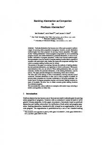
always @(posedge clk) begin ... if ( v > 1024 ) begin if (...) set the error bit; end ... v = v + x ; end

Figure 2: Precomputing candidates of visible variables. In other words, we bypass the step of first generating new predicates based on WP-based analysis. This is because in the subsequent refinement iterations, it is likely that a large number of new predicates (corresponding to the WP of P l ) are needed, due to the nature of v’s transition function. In Fig. 2, for instance, if the predicate (v