The final publication is available at Springer via http://dx.doi.org/10.1007/s12083-013-0205-7
Hybrid Fluid Modeling Approach for Performance Analysis of P2P Live Video Streaming Systems Zoran Kotevski · Pece Mitrevski
Abstract In this paper, a hybrid modeling approach with different modeling formalisms and solution methods is employed, in order to analyze the performance of peer to peer live video streaming systems. We conjointly use queuing networks and Fluid Stochastic Petri Nets, developing several performance models to analyze the behavior of rather complex systems. The models account for: network topology, peer churn, scalability, peer average group size, peer upload bandwidth heterogeneity and video buffering, while introducing several features unconsidered in previous performance models, such as: admission control for lower contributing peers, control traffic overhead and internet traffic packet loss. Our analytical and simulation results disclose the optimum number of peers in a neighborhood, the minimum required server upload bandwidth, the optimal buffer size and the influence of control traffic overhead. The analysis reveals the existence of a performance switch-point (i.e. threshold) up to which system scaling is beneficial, whereas performance steeply decreases thereafter. Several degrees of degraded service are introduced to explore performance with arbitrary percentage of lost video frames and provide support for protocols that use scalable video coding techniques. We also find that implementation of admission control does not improve performance and may discourage new peers if waiting times for joining the system increase. Keywords Modeling, Performance, Live video streaming, Peer to Peer, Queuing networks, Fluid Stochastic Petri Nets, Discrete-event simulation Z. Kotevski () · P. Mitrevski Department of Computer Science and Engineering Faculty of Technical Sciences University of St. Kliment Ohridski Ivo Lola Ribar bb, 7000 Bitola, R. Macedonia e-mail:
[email protected] P. Mitrevski e-mail:
[email protected]
1 Introduction The use of Internet video streaming services is spreading rapidly and web technologies for live video broadcast increasingly attract more and more visitors. In the classical client/server system architecture, the increase in number of clients requires more resources like high bandwidth transmission channels (TCs) with large upload rates. Since these TCs are extremely expensive, the usual outcome is a limited number of Unicast connections that a Streaming Server (SS) can support at a given time. In the early nineties, it was expected that IP Multicast [1] will be the natural technology to satisfy the requirements of large scale streaming with lower cost. However, the lack of support for higher level functionality, scalability issues and requirements for hardware Internet technology changes, have prevented its wider deployment. This motivated the science community to work in the field of new approach for Internet Live Video Streaming (LVS) by the use of Peer to Peer (P2P) networking technologies. In essence, P2P LVS systems are data dissemination logical networks formed on top of the physical network. Basically, they form two different types of logical topologies: tree and/or mesh [2]. While the tree topology forms structured network of a single tree such as Nearcast [3], or multiple multicast trees as in [4], mesh topology is unstructured and does not form any firm logical construction, i.e. it organizes peers in swarming or gossiping-like environments, such as Chainsaw [5] or CoolStreaming [6]. Some protocols use a combination of these two aspects, forming a hybrid network topology, such as [7,8,9,10,11]. In mesh systems peers are organized in groups or neighborhoods and every peer maintains connections with all the peers from its group. The video data is divided in small pieces called chunks that are streamed by the source (SS) to the peers. Each peer acts as a server as well as a client, forwarding received video chunks after some short buffering. Chunk requesting and forwarding is controlled by a chunk scheduling algorithm,
which is responsible for on-time chunk acquisition and delivery among the neighboring peers. The peers join and leave the network at free will (peer churn) which has a negative effect on system’s performance. Another complication is added by the peers’ Upload Bandwidth (UB) heterogeneity. Hence, in the last decade, a number of such protocols were developed. In this manner, CoolStreaming [6] have reported a number of 4,000 concurrent users and Gridmedia [12] reported more than 15,000. Recent measurement study of PPLive [13] reported a peek of even 200,000 simultaneous users (when on January 28, 2006, PPLive broadcasted the annual Spring Festival Gala on Chinese New Year), with bitrates in range of 400 – 800 kbps, which corresponds to an aggregate bitrate of ~100 gbps. Clearly, these P2P LVS networks offer huge economic benefit in deploying and managing IP video streaming, but these systems are still in their early stages and bring a lot of open issues and research challenges that need to be explored. Therefore, prior to creating a P2P LVS system, it is necessary to analyze its behavior via representative model that provides deeper insight into system’s performance, gathering valuable information for design and development of such systems. Modeling and performance analysis of P2P LVS systems is a challenging task which requires addressing many properties and issues of P2P systems that create complex combinatorial problem. Following a number of approaches in which different modeling formalisms and solution methods are combined in order to exploit their complementary strengths, in this paper, a hybrid modeling approach with different modeling formalisms and solution methods is employed, in order to analyze the performance of P2P LVS systems. We conjointly use queuing networks (QNs) and Fluid Stochastic Petri Nets (FSPNs) [14,15,16], developing several performance models to analyze rather complex peer to peer streaming systems. What needs to be mentioned is that, in FSPNs, the fluid variables are represented by fluid places, which can hold fluid rather than discrete tokens. Transition firings are determined by both discrete and fluid places, and fluid flow is permitted through the enabled timed transitions in the Petri Net. By associating exponentially distributed or zero firing time with transitions [15], the differential equations for the underlying stochastic process can be derived. In our study, a QN model is used to obtain a comparable analytical solution for a bufferless system, while for the FSPN model of both bufferless and buffered system, only simulation solution method appeared to be feasible. The models unite numerous features of P2P LVS systems, such as network topology, peer churn, scalability, peer average Group Size (GS), peer UB heterogeneity and video buffering, as well as several features unconsidered in previous performance models such as Admission Control (AC) for lower contributing peers, control traffic overhead and internet traffic packet loss.
The rest of this paper is organized as follows. Section 2 presents our main motivation and gives an adequate review of related work. In section 3 the model definition is presented, starting with a general overview of the modeling idea. Following is a description of peer churn along with the transfer of bits as a fluid stream through the network. Later, the stream function is derived and closed form expressions for QN model of bufferless system are obtained. Next, the FSPN models for a system with buffering and a system that accounts for AC are described. In section 4, performance evaluation results and analyses are presented accompanied with brief discussions regarding a handful of key elements. Section 5 provides concluding remarks and summary of contribution.
2 Motivation and related work Several related articles use fluid models for performance analysis of file sharing P2P systems. Qiu D. et al. [17] modeled mesh based, file sharing P2P system, developing simple deterministic fluid model that provides some insights in the system’s performance. Yue Y. et al. [18] developed a general fluid model to study the performance and fairness of BitTorrent-like networks. In its basics, this model is an extension of [17], taking in consideration the diversity of peers’ bandwidth capacities. Perronnin FC. et al. [19] proposed a stochastic fluid model for performance analysis of Squirrel, a P2P cooperative Web cache, where under the assumption that all objects are equally popular, they provide closed form expressions to model file sharing system where peer churn is modeled as an M/M/∞ Poisson process. The model is extended to include unequal popularity by grouping the documents into classes and implementing the same steady state solution. Similar approach is used to model P2P Video on Demand (VoD) systems. Tu YC. et al. [20] presented an analytical framework to quantitatively study the features of a hybrid VoD streaming model that involves Content Delivery Network (CDN) and P2P technologies. Yazici MA. et al. [21] introduce Markov chain based model to study mesh based, multi-stream, P2P VoD systems. The model accounts for peer churn, and query and setup times for a new connection with exponential probability distribution, while Lu Y. et al. [22] presented an analytical fluid model for mesh based P2P VoD system. The models in [17-20,22] are described by sets of differential equations, solved in steady state, and the accuracy of the models in [19,20] is validated by a comparison to discrete event simulations (DESs). Concerning the live video streaming, inspired by [17], Tewari S. et al. [23] proposed an analytical model for BitTorrent based P2P LVS system that concentrates on the number of fragments available for sharing, fragment size and optimal GS. Zhou Y. et al. [24] developed a simple stochastic model for comparing different data driven downloading strategies for P2P LVS systems in symmetric
network settings. The model is defined by differential equations in discrete and continuous case that are solved numerically and evaluated by simulations. Wu D. et al. [25] developed infinite-server queuing network models to analytically study the performance of P2P LVS systems. Their analytic models capture the essentials of multichannel video streaming systems taking into account: channel switching, peer churn, peer UB heterogeneity and channel popularity. Liu F. et al. [26] developed mathematical model to study the inherent relationship between time and scale in P2P LVS systems during a flash crowd. The model shows that system scaling behavior and peer startup delay are strongly affected by different peer arrival patterns and peer churn. Kumar R. et al. [27] developed stochastic fluid theory for mesh based P2P LVS systems. It represents general base for modeling such systems while interpreting peer churn as multiple levels M/G/∞ Poisson processes and adopting fluid flow model for video streaming, The analyses include modeling a churnless bufferless system, bufferless system with churn, and P2P LVS system model with peer churn and buffering, while its analytical expressions bring insights in service degradation in all these cases. The performance of the P2P system, as the joining rate of new peers becomes very large, is studied and explicit expressions for the probability of degraded service for large systems are obtained. Wu J. et al. [28] proposed an extension of [27] focusing on the problem of maximizing Universal Streaming (US) rate in P2P LVS systems with a difference in taking in consideration neighborhood constraints. The model is restricted by assumptions of a churnless, bufferless system and peers with homogeneous UBs. Even though works in [17-22] represent inspiration to model such systems, since they deal with file sharing or VoD, their models are not applicable to P2P LVS systems. Although in [27] multiple features of these systems are considered, such as peer churn, buffering and heterogeneity of peers’ UB, peer GS is not taken into account. The other models concentrate on a very limited number of system characteristics. The models in [23,24,28] do not consider peer churn which is one of the most important aspect of P2P LVS systems, and [25,26,28] consider only bufferless systems. However, beside the existing deficiencies, none of the presented models account for control traffic overhead and Internet traffic packet loss, and their influence on system performance. They also do not provide information about service degradation, the minimum required SS UB, the optimum video stream rate for a given scenario, the performance boost gained if AC for low contributing peers is used, nor the average waiting time for admission controlled peers. In this paper we combine multiple features of P2P LVS systems in a hybrid approach using QNs, and FSPNs developing fluid models that provide an in-depth insight into the system’s performance in a variety of scenarios. We base our model on [27] and extend it to include features that are not considered in previous researches. For the
solution of the QN model a closed form expression is derived, and for the FSPN models the solution is provided by DESs. Hence, we can summarize our contribution as follows: 1. This is the first modeling approach for performance analysis of P2P LVS systems that, at the same time, accounts for so many features of these systems, including: i) network topology, ii) peer churn, iii) scalability, iv) peer average GS, v) peer UB heterogeneity and vi) video buffering, while, for the first time, accounting for vii) control traffic overhead, viii) internet traffic packet loss and ix) AC for lower contributing peers. 2. The analysis discloses: i) optimal peer GS, ii) optimal buffer size, iii) system’s performance with respect to scaling and iv) influence of the control traffic overhead, while introducing several new output parameters, such as: v) minimum required SS UB, vi) several degrees of Quality of Service degradation (Δ), to explore system’s performance with an arbitrary percentage of lost video frames, vii) optimal video rate for known peers’ average UB and viii) performance evaluation of a system that implements AC, where the average number and the average waiting time for admission-controlled peers are presented, as well. 3. To the best of our knowledge, this is the first effort that uses FSPNs for modeling such systems, while at the same time introduces a novel DES approach for simulating FSPNs using process-based discrete-event simulation language.
3 General model definitions The art of modeling and performance analysis covers two simple aspects. First, the model should always be simple, intuitive and close to designer’s intuition of what the modeled system looks like. Second, it should account for as many features as possible, while providing accurate performance results without compromising its simplicity. We consider a P2P LVS system that adopts mesh topology, where peers are randomly organized into groups or neighborhoods, and each group member communicates with all his neighbors exchanging video chunks. The model also incorporates peers’ UB heterogeneity that is implemented by classifying peers in several classes based on their UB capabilities. We define that the lowest contributing peers (class 1) have UB of P1UB, and the highest contributing peers (class n) have UB of PnUB. Depending on the number of peer classes against which we want to evaluate the system’s performance, the UBs of peers from the in-between classes are calculated by Eq. (1).
PiUB P i 1UB
PnUB P1UB # Cls 1
(1)
where: PiUB – UB of class i peers #Cls – Number of classes where #Cls> 1 We assume asymmetric network settings where peers have infinite download bandwidths (DBs) and therefore peer’s download capabilities are not taken in consideration. Peer arrival is described as a stochastic process with exponentially distributed interarrival times, with mean (1/λ), where λ is the arrival rate. Different from [27], where no assumptions on the peers viewing times distribution were made, we assume exponentially distributed viewing times with mean duration of “T” minutes. Clearly, since each peer is immediately served after joining the system, we have an M/M/∞ queuing model with infinite number of servers and exponentially distributed joining and leaving rates. For such a model, the mean service time (T) is T = 1/μ, where µ is the departure rate. Now, λ represents peer arrival in general, but the peers from different classes do not share the same occurrence probability (pi). So, class 1 peers arrive with rate λ1=p1 * λ, class 2 peers arrive with rate λ2=p2 * λ, and class n peers arrive with rate λn=pn * λ, where p1 + p2+ … + pn = 1. This way the model with peer churn is represented by several independent M/M/∞ Poisson processes, one for each peer class. The average number of peers that are concurrently served in the system as a whole is given in Eq. (2).
i i1 n
(2)
where ρi is the average number of class i peers that are concurrently served, and ρi={λi/µ: i=1,2,…,n}. The exponentially distributed peer interarrival times have already been experimentally confirmed by Sripanidkulchai K. et al. [29], but exponentially distributed peer viewing times (session durations) may seem like a strong assumption, since in this same experimental research [29] it is concluded that session durations follow heavy-tailed distribution, or more specifically Pareto distribution. For this reason we present two arguments that explain the rationale behind this assumption and why it does not jeopardize the correctness of the results obtained. Namely, the use of exponentially distributed firing time has been regarded as a restriction in the application of Petri Net based models. There are many phenomena whose times to occurrence are not exponentially distributed, but the hypothesis of exponential distributions, allows the construction of models which can give a more qualitative rather than quantitative analysis of real systems. The inclusion of non-exponential distributions destroys the memoryless property of the associated marking process, and further specification is needed at the Petri Net level in order to uniquely define how the marking process is conditioned on the past history. The memoryless property
characterizes many natural processes and therefore the exponential distribution is widely used in modeling and analysis of stochastic systems. At last, but not least, the research of Ou Z. et al. [30] deals with the effects of different churn models on the performance of structured P2P networks. More specifically, exponential, Pareto and Weibull distributions are used to provide comparative analysis, and throughout extensive simulations they conclude that the simulated different churn models do not have a significant effect on the performance of the simulated P2P systems. Their performance curves show that models that use exponential and Pareto distributions act nearly identically, and Weibull models exhibit only slight difference. As for the streaming part of the model, we adopt fluid flow, where bits are represented as atoms of fluid that travel through fluid pipes (network infrastructure) with rate dependent on the system’s condition. We identify four separate fluid flows (streams) that travel through the network with different bitrates. The main video stream represents the video data that is streamed from the source to the peers, further stated as video rate (VR). The second stream is the play stream which is the stream at which each peer plays the streamed video data, further stated as play rate (YR). One of the characteristics that make this model widely different than others is the implementation of control traffic overhead. This is the third stream, simply named as control rate (CR), which describes the exchange of control messages needed for the logical network construction and management. In the majority of research articles, CR is represented as a percentage of the total traffic [6] or percentage of the video rate [31]. We disagree with both conventions for expressing the CR because, according to [6,7], CR is independent of the VR or other traffic and rises linearly with GS. Therefore, we propose that it is more convenient to express CR in pure bitrate units of kbps. These conclusions also imply that there is an equivalency between CR and GS, i.e. GS is implicitly modeled via the definition of CR. For example, CR of 2.4 kbps implies an average group size of 60 peers, CR of 4 kbps implies that peers are organized in groups with an average size of 100 peers, etc. More details about the control rates and their corresponding GSs can be found in Section 4.3 and Table 5. The fourth stream that has also never been included in previous researches is the network infrastructure packet loss. According to [32], an average of 15% of all traffic is lost and therefore needs to be resent. We denote this stream as loss rate (LR) and the percentage of lost packets as loss percentage (LP). In the remainder of this study LP is set at 15% throughout all the presented analyses. Finally, in several model variations, we incorporate AC for peers that contribute less resource than their requirements. For all the scenarios we calculate the Δ probability and, in some scenarios, we introduce several degrees of Δ. Stream delay, peer selection strategies and chunk size are not taken into account.
3.1 The stream function ψ()
Lp
In [27], the fluid function φ() is defined as the maximum achievable rate that can be streamed to any individual peer at a given time (Eq. 3). This fluid function depends on the SS UB, the number of participating peers and their UBs. n SUB # Pi PiUB i 1 min SUB , n # Pi i 1
() then Since, () CR LR VR and LR 100
V CR Lp () , i.e. () R () VR C R 1 LP 100 100
(3)
□
For further simplification we denote (VR + CR)/(1 – LP/100) as “RMIN” i.e. the minimum streaming rate to each individual peer required to achieve US.
where, SUB – SS UB #Pi – The number of class i Peers 3.2 Modeling the buffered system Hence, the US is achievable if and only if φ() ≥ VR. For more detailed explanation of φ() and US we refer the reader to [27]. To satisfy the requirements of our models we define a new function that we refer to as the stream function ψ(). The stream function is not the maximum, but rather the actual rate that is streamed to any individual peer at any given time. The stream function ψ() is limited by the fluid function φ() and ψ() ≤ φ(). Theorem 1: In our models US is achievable if and only if:
V C R () R L P 1 100
(4)
Proof: We can imagine the whole system as a fluid infrastructure where the stream function ψ() tries to deliver enough fluid for three consumers (LR, CR and YR). LR and CR have the priority over YR, so if there is enough fluid flow for YR to be equal to VR the principle of US is preserved. Otherwise, if YR drops below the value of VR, the system operates in Δ mode. So, to achieve US, ψ() must be greater or equal to (CR + LR + VR).
Fig. 1 Bit transfer through the P2P LVS network
In this section we describe the bit transfer (fluid flow) from the SS buffer (SB) to each peer’s buffer (PB). For this purpose we adopt the “latest useful chunk” scheduling strategy implemented at the SS. This way the SS always tends to send the latest received useful chunk to the new peer, thus assuring that the freshest video content is the first that is sent to the peers. The idea is presented in Fig. 1, where all the buffers are represented as buckets that can contain fluid and the fluid transfer media is a stream pipe (SP). The SS copies bits from the SB and forwards them throughout the SB’s outflow SP with rate equal to the stream function ψ(). At the same time, since the stream delay is not taken in consideration, each PB receives bits at the same rate of the stream function through its inflow SP. For this reason we imagine that all stream pipes are “firmly interconnected” and can move up or down together according to the system’s conditions. The video stream is generated at the SS and the SB is filled with fluid at rate VR. Fluid enters at the top of the SB and it is drained at the bottom at the same rate as the inflow rate (VR). SB is always full and the fluid travels through the SB with rate VR from the top to the bottom. SB’s outflow SP copies the bits from the SB at its momentary position and streams them as a fluid with rate ψ().
The crucial thing in this copying and forwarding of bits is that the vertical movement of all SPs depends on the stream function ψ(). When ψ() drops below the required value for US i.e. when ψ() < RMIN, the bits are traveling down the SB faster than they can be copied and forwarded through the SB’s outflow SP. Consequently, since the system does not want to miss any bit, the SPs move down to be able to replicate and forward every single bit. The speed at which the SPs travel down is proportional to the stream function ψ(). The smaller the stream function ψ(), the faster the stream pipes travel down. Oppositely, when SPs are in a lower position and ψ() > RMIN, they travel up. This pipe movement has its limitations. The SPs can move up or down from the bottom of the buffers to their top. US is challenged only when the SPs are at the bottom of the buffers (PBs are empty) and ψ()< RMIN. In the meantime, a PB is filled with rate ψ() and drained with rate (YR + LR + CR), where LR and CR have the priority over YR. When ψ() drops below the value of RMIN, the SPs travel down and the level of fluid in each PB is dropping. When ψ() rises above the value of RMIN, SPs travel up and the level of fluid in each PB is rising. The level of fluid amount in each PB corresponds to the position of the PB inflow SP. Again, US is challenged only when PBs are empty and ψ() < RMIN, i.e. when YR < VR. Since the SB outflow pipe and all PBs inflow pipes are “interconnected” they move up/down simultaneously. This modeling approach provides us the unique possibility to model the whole system by the behavior of the fluid level in a single PB. The pipe movement represents fluid level changes in the PBs and YR defines whether US is achievable. If the system is able to achieve for YR to be equal to VR US is preserved. When YR drops below the value of VR the system is experiencing Δ. 3.3 Queuing network model QN model is used to develop analytical expressions for performance evaluation of bufferless systems. We modeled the system as a QN with several independent M/M/∞ queuing (Poisson) processes for the different peer classes. The underlying continuous time Markov chains are birthdeath processes where, as elaborated previously in Section 3, the mean number of class i peers, that are concurrently being served in the system, is ρi={λi/μ :i=1,2,..n}. The state space “S” describes all the possible states of the QN model, where S = {sj: j=1,2,…,m}. sj is a row vector representing the number of peers present in each queue, for a given system state. In this case, the number of peers from a certain class i that are present in the system follows a Poisson probability distribution, which assigns non-zero probabilities to the region ± ρi from the mean. Therefore, a good approximation of the maximum number of class i peers that could concurrently be present in the system is 2ρi. We derive the expression for calculating the approximate value of the number of all possible states “m”, which is given in Eq. (5).
m
n
2
1
i
(5)
j 1
where the “+1” is added to count the state when no peer is present in the queue. Clearly, the state space of our QN model is extremely large. Even for a small system with an average of 100 peers, where peers are classified in four classes that evenly participate, the number of all possible states exceeds 6x10⁶. However, we derive the steady state equations from the queuing theory where the steady state probability for k peers of class i, to be present in the system is given in Eq. (6).
Pi (k )
ik k!
e i
(6)
When calculating the Poisson probability for large systems, because of the large numbers that occur due to the factorial present in the formula, the presented analytical solution in Eq. (6) did not appear to be feasible. Hence, using the Central limit theorem we approximated the Poisson probability distribution with Normal probability distribution, where the steady state probability for k peers of class i to be present in the system is given in Eq. (7).
Pi (k )
1
e
2i
k i 2 2 i
(7)
For the extent of accuracy in this approximation we turn to the Berry-Esseen theorem which is more deeply discussed in the research of Korolev V. and Shevtsova I. [33], where the best so far known upper estimate of the absolute constant (C) in the classical Berry-Esseen inequality is proven to be: C ≤ 0.4784. Thus, the maximum relative error (δr) of the Normal approximation to the Poisson distribution in this case is given in Eq. (8).
r
C min i
(8)
Later, in Section 4, using the Normal approximation, we evaluate the performance of a large system with ρ = 104 peers, of which the least participating class of peers has ρi of 1500. Hence, the relative error of our approximation exhibits an upper bound of 0.01235 which yields a degree of accuracy ≥ 98.765%. Now, since we have several independent Poisson processes the probability for the system to reach certain state sjS is given in Eq. (9). n
P S [i]
P Sj
i
i1
j
(9)
where "Sj[i]" shows the number of peers in queue i when the system is in the state j. For the bufferless system, we can group all possible system states in two groups: states that support US, and states in which the system operates in Δ mode (as in Theorem 1). Thus the overall probability for US is given in the following Eq. (10):
PUS
m
P(S ), P(S ) : () R j
j
MIN
(10)
j 1
and Δ probability is: P 1 PUS
(11)
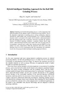
3.4 FSPN model General FSPN model of P2P LVS system with buffering is shown in Fig. 2. The model has n discrete places (single line circles), n+5 timed transitions (rectangles), n immediate transitions (short lines) and a single fluid place depicted by means of two concentric circles. Discrete places are connected with discrete arcs that are drawn with single lines through which tokens are transferred. Fluid arcs, through which fluid is pumped, are drawn as double lines to suggest a pipe. Peers are represented as discrete tokens and video stream is represented as fluid flow. Discrete tokens join and leave the discrete places via discrete arcs. The fluid is pumped through fluid arcs and is streamed to and out of the fluid place. The model’s unique fluid place PBUF represents a single PB. TA is a timed transition with exponentially distributed firing times that represents peer arrival, which upon firing (with rate λ) puts a token in PCS. PCS (representing the control server) checks the token class (peer class) and immediately forwards it to one of the discrete places P1,
Fig. 2 FSPN model of P2P LVS system
P2, P3…Pn. These places represent the peer classes of our P2P LVS system. The transitions that forward tokens to the discrete places are TJ1, TJ2, TJ3…TJn. These are immediate transitions that (when there is a token in PCS) fire with probabilities p1, p2, p3… and pn respectively. These probabilities multiplied by λ represent the rates of occurrence of a peer from certain class, where p1 + p2 +…+ pn= 1. Transitions TL1, TL2, TL3…TLn are enabled only when there are tokens in discrete places P1, P2, P3…Pn respectively. These are marking dependant transitions, which, when enabled, have exponentially distributed firing times with rate μ·#Pi. Upon firing they take one token out of the discrete place to which they are connected. Also, these transitions, when enabled, pump fluid through the fluid arc to the fluid place. Flow rates of ψ() are piecewise constant and depend on the number of tokens in the discrete places and their class. Continuous place PBUF represents single peer’s buffer. It is constantly filled with rate ψ() and drained with rate (YR + LR + CR). ZBUF represents the amount of fluid in PBUF and ZBUFMAX is the buffer’s maximum capacity. Since we have only one fluid place the process of fluid level changes in PBUF can be described by first order, ordinary linear differential equations given in Eq. (12). Transition TS represents SS functioning. It is always enabled (except when there are no tokens in any of the discrete places) which means that it constantly pumps fluid into the continuous (fluid) place PBUF. Transition TPLAY is also always enabled and constantly drains fluid from the continuous place PBUF, with play rate YR. YR tends to be equal to VR except when the system works in Δ mode. Other transitions that are always enabled are TLOSS and TCONTROL and constantly drain fluid from the fluid place PBUF, with rates LR and CR respectively.
Priorities (pr1, pr2 and pr3) are assigned to transitions TLOSS, TCONTROL and TPLAY, respectively, in descending order. TLOSS has the priority over both TCONTROL and TPLAY, whereas TCONTROL has the priority only over TPLAY. The lowest priority (pr3), assigned to TPLAY, means that when the stream function ψ() does not have the capability to fully support all these three streams, i.e. when ψ() < RMIN, the rate of YR is the first to drop. The number of all possible discrete states of this FSPN model is extremely large (Eq. (5)). However, even though we deal with immense state space, it is not difficult to identify 4 distinct cases of grouped states presented in Table 1. These cases are a mix of states of the discrete part and states of the continuous part of the net.
0 dZ BUF t () VR LR CR dt () VR LR CR 0
case1, case2, case3,
(12)
case4.
Table 1 Cases of system states
case1
if
case2
if
case3
if
case4 if (Δ mode)
ZBUF = ZBUFMAX and φ() ≥ RMIN 0