Feb 6, 2009 - [2] C. von Campenhausen, I. Riess, and R. Weissert, J. Comp. Physiol. A 143, 369 (1981). [3] S. Coombs, R. Anderson, C.B. Braun, and M.
week ending 6 FEBRUARY 2009
PHYSICAL REVIEW LETTERS
PRL 102, 058104 (2009)
Hydrodynamic Object Recognition: When Multipoles Count Andreas B. Sichert, Robert Bamler, and J. Leo van Hemmen Physik Department T35 & Bernstein Center for Computational Neuroscience-Munich, Technische Universita¨t Mu¨nchen, 85747 Garching bei Mu¨nchen, Germany (Received 21 May 2008; revised manuscript received 15 December 2008; published 6 February 2009) The lateral-line system is a unique mechanosensory facility of aquatic animals that enables them not only to localize prey, predator, obstacles, and conspecifics, but also to recognize hydrodynamic objects. Here we present an explicit model explaining how aquatic animals such as fish can distinguish differently shaped submerged moving objects. Our model is based on the hydrodynamic multipole expansion and uses the unambiguous set of multipole components to identify the corresponding object. Furthermore, we show that within the natural range of one fish length the velocity field contains far more information than that due to a dipole. Finally, the model we present is easy to implement both neuronally and technically, and agrees well with available neuronal, physiological, and behavioral data on the lateral-line system. DOI: 10.1103/PhysRevLett.102.058104
PACS numbers: 87.85.Ng, 47.90.+a, 87.19.lt
All fish and some aquatic amphibians possess a unique sensory facility, the lateral-line system. This system is composed of mechanosensory units called neuromasts located on the trunk of the animal. They consist of small cupulae, gelatinous flags protruding into the water, which are sensitive to the local water velocity [1]. Aquatic animals use their lateral-line system to localize predator, prey, obstacles, or conspecifics. The lateral line enables even blind fish to navigate efficiently through their environment and discriminate different structures and obstacles [2]. It is supposed that aquatic animals analyze the hydrodynamic structure of the velocity field to determine size, speed, and presumably shape of the object generating it [2,3]. This can be done even indirectly, for example, through the wake [3]. The question we now pose, and answer, is whether and how a passive detection system such as the lateral line can both localize a moving object and determine its shape in an incompressible fluid such as water, or air at low velocities. Passive localization has several advantages over active localization such as not getting noticed by the object you observe and being far less energy consuming. Most studies, both experimental and theoretical [4,5], used a vibrating or translating sphere as a stimulus. Because of the special symmetry of the sphere, the resulting velocity field is exactly that of a dipole—no matter whether vibrating or translating [6]. Of course, not all objects in nature are spheres. Only for vibrating bodies could one identify [7] the influence of their shape on the flow field, showing a reasonable dominance of the dipole. The literature lacks, however, a general explanation in a more general setting. In this Letter, we show how much, or little, information is available in the velocity field, how one can extract it, and to what extent it depends on the distance. More, in particular, we show how hydrodynamic object characterization in terms of a mathematical description in three dimensions is possible by means of a multipole 0031-9007=09=102(5)=058104(4)
expansion (ME). In addition, we show how an aquatic animal, called a detecting animal (DA), such as a predator, can read out the velocity field and reconstruct the shape of a stimulus, viz., a submerged moving object (SMO), such as prey; cf. Fig. 1. A velocity field vðrÞ ¼ �r�ðrÞ represents an adequate and natural stimulus to the lateral-line system and can be described by a multipole expansion of the velocity potential �ðrÞ [6] because the relevant fluid dynamics is well described by the Euler equation [8]. Using the R real spherical harmonics Ylm and the multipole moments q ¼ ð. . . ; qlm ; . . .Þ, we can expand the velocity potential �, �¼
1 X l X l¼1 m¼�l
qlm �lm ¼
1 X l X l¼1 m¼�l
qlm
R 1 Ylm ð�; ’Þ : 2l þ 1 rlþ1
(1) For the sake of simplicity, we focus on rotationally symmetrical bodies whose surface S can be described through coordinates & 2 ½0; �� and � 2 ½0; 2��, 1 0 �1=3 � � �B pffiffi2 sinð�=2Þ sinð&Þ cosð�Þ C &� B ��1=3 C C: (2) B pffiffi Sð&; �Þ ¼ N cos �3 @ 2 sinð�=2Þ sinð&Þ sinð�Þ A �2=3 cosð&Þ
FIG. 1 (color online). Submerged moving objects (SMOs) appear in widely varying shapes. Furthermore, aquatic stimuli may, but need not move at all, for example, vortex structures that are generated in the wake of a swimming fish or at the end of the fins [3]. These stimuli imprint information on the flow field that can be read out by the lateral-line organs [10].
058104-1
Ó 2009 The American Physical Society
PHYSICAL REVIEW LETTERS
PRL 102, 058104 (2009)
The parameters � 2 ð0; �=2� and � 2 ð0; 1Þ determine the shape of the surface. We note that vortex structures can be described by means of an ME as well [6]. Because of the Euler equation, only the Neumann boundary condition v � nS ¼ 0 is realizable where nS denotes a normal vector to the surface S. In terms of spherical coordinates, we can calculate the components of vðrÞ ¼ �r�ðrÞ ¼ ðvr ; v� ; v’ Þ at r through coefficients arlm , etc., so that vr ¼
1 X l X
qlm arlm ;
v� ¼
l¼1 m¼�l
1 X l X l¼1 m¼�l
v’ ¼
1 X l X
qlm a�lm ; (3)
qlm a’lm :
l¼1 m¼�l
The equations (3) can be written in matrix form v ¼ Aq with the matrix A containing the known coefficients arlm . To explicitly calculate the single multipole moments qlm , we have to specify the boundary condition with respect to nS and, for the sake of simplicity, the uniform speed v1 of the SMO in the stationary frame of reference. The boundary condition then reads
week ending 6 FEBRUARY 2009
obvious that plankton, which is ten to a hundred times smaller than the DA, will not transmit any shape information through the flow field—and in this case shape information is not needed either. However, as stated before, in schooling, mate finding, or predator-prey behavior object information can make a difference. Moreover, as shown in Fig. 2, different shapes are represented by different sets of multipole moments. How, then, can aquatic animals such as fish reconstruct the above multipole moments from water velocity measured through their lateral-line system? Of course the animal has to fulfill this task under the influence of omnipresent noise and the limitations of its neuronal system. Our reconstruction model for three-dimensional shape recognition is based on a maximum-likelihood estimator [11]. That is, we are looking for the multipoles q with the highest probability given the measured velocities w on the DA’s body. So to speak, this estimator maximizes the conditional probability pðq; r0 jwÞ for the SMO’s center of mass r0 , which also has to be determined by means of the information available through the DA’s superficial neuromasts, the water velocities. The velocity size wi at organ i is given by wi ¼ T ðr0 ; ri Þq þ ni .
v ðrS Þ � nS ¼ nS � v1 ¼ nS T AðrS Þq with rS 2 S: (4) The influence of the multipoles in (3) decreases with increasing l. Hence we expand the velocity field only up to a certain number k and set qlm ¼ 0 for l > k. We are thus ^ To find the dealing with an approximation, denoted by q. best approximation, we take several positions 1 � i � n randomly distributed on an SMO surface and calculate the associated surface normals ni , the matrix Ai , and write it line by line into the matrix T :¼ ð. . . ; ni T Ai ; . . .Þ. The index i of the velocity components wi :¼ v1 � ni of the vector w corresponds to ni and therefore labels the same position. To calculate the multipoles we simply solve the linear equation T q^ ¼ q. The multipole moments follow from q^ ¼ ðT T T Þ�1 T T w [9]. The solution approximates the multipole coefficients up to a given k optimally in the sense of minimal quadratic error. Introducing a characteristic length scale �, say the body length of the SMO, into Eq. (1) we get X v ðrÞ ¼ qlm ð�=rÞlþ2 flm ð�; ’Þ; (5) l;m
where flm ð�; ’Þ are functions depending only on the angular � and ’ coordinates and can be calculated by means of (1). In doing so, we obtain dimensionless multipole moments. On the one hand, we can compare them independently P of the SMO size. On the other hand, we see from vðrÞ ¼ l;m ð�=rÞlþ2 qlm flm ð�; ’Þ how the influence of each multipole varies in dependence upon the size � of the SMO and the distance r to the DA. This result tells us that the shape of the SMO is only important if the size � and the distance r are of the same magnitude. It is, e.g.,
FIG. 2. Different shape parameters result in distinguishable sets of multipole components even for l � k ¼ 3 in (3); � increases along the vertical axis and � along the horizontal one. We have calculated q^ through a raster of 30 000 randomly distributed positions on each moving object’s surface and used objects with length of about 5 cm and a matching moving speed v1 ¼ 0:01 m=s. Each volume is normalized to the volume of the unit sphere. It is therefore fair to say that the dipole stays almost constant while q20 varies according to � and q30 to �. The relative error 4ðkÞ :¼ jT q^ � wj=jwj on S as calculated for rotationally invariant elliptic bodies gives 4ðkÞ < 0:4 for k ¼ 3 and � < 2. It converges slowly to about 0.15 for k ! 1. For � � 2 a multipole expansion cannot describe the correct velocity field. This, however, is not too restrictive. For example, the fish in Fig. 1 can be described by � � 1 (left fish) and � � 2 (right fish).
058104-2
PRL 102, 058104 (2009)
week ending 6 FEBRUARY 2009
PHYSICAL REVIEW LETTERS
We note that the matrix T ðr0 ; ri Þ depends on the SMO position r0 and the position ri of the lateral-line organ i (DA). Noise is modeled by adding independent Gaussian random variables ni with mean 0 and standard deviation �n to the wi . All positions r0 are of equal probability. We therefore take a Gaussian probability distribution pðq; r0 Þ � expð�q2 =2�2q Þ. Instead of maximizing the combined probability based on Bayes law, we maximize its logarithm Lðq; r0 Þ :¼ ln½pðq; r0 jwÞ�. Defining � :¼ �n =�q , we just have to maximize Lðq; r0 Þ ¼ �f½w � T ðr0 ; ri Þq�2 þ �2 q2 g
(6)
with respect to the multipole-moment vector q and r0 . The necessary condition for a maximum of the likelihood ^ r^ 0 Þ at the correctly estimated position r^ 0 is Lðq; @L ðq; r^ 0 Þjq¼q^ ¼ ½ðT T T þ �2 Þq � T T w�jq¼q^ ¼ 0; (7) @q which leads to a linear system of equations solvable by means of the pseudoinverse technique [9], q^ ¼ ðT T T þ �2 Þ�1 T T w:
(8)
We estimate the set of multipoles q^ given only the measured velocities w at the lateral-line organs. A neuronal implementation of these calculations is straightforward and can be done easily by neuronal hardware; see Fig. 3. Thus the position and the appropriate multipole moments can be calculated neuronally. To test whether it is possible for aquatic animals using the above method to determine SMO’s position and shape, we have applied noise to the input signal wi . We have used �n ¼ 10�4 m=s as standard deviation of the noise, which corresponds to the velocity threshold of Xenopus’s lateralline organ [1]. Furthermore, we define a signal-to-noise ratio, SNR :¼ v1 =�n , that dominates the performance as compared to the number of neuromasts, cf. [12]. The more
FIG. 3. Neuronal implementation of (8) is straightforward. In a first step ðAÞ ! ðBÞ the multipole components q^ lm ðr0 Þ (B) are calculated for different positions r0 from the measured water velocities wi at the neuromasts (A). This corresponds to a network of synaptic connections between the lateral line and the central nervous system. The strength of the individual connections can be computed from the entries of the right-hand side of (8) or can be learned neuronally [14]. In a second step ðBÞ ! ðCÞ, Lðq; r0 Þ is calculated from the q^ r0 , which can also be done ^ r^ 0 Þ by feedforward connections, cf. (6). The maximum Lðq; indicates the correct position of the SMO and selects the optimal q^ r0 from step ðCÞ ! ðBÞ, cf. (7).
multipoles we use, the more positions are of high probability because one has more parameters to fit the measured wi ’s. Thus the estimated position gets ambiguous but the shape estimate improves. Choosing the right � for a certain k can compensate this effect and enables a faithful localization. In Fig. 4 we show the ability of our method to estimate the SMO position r^ 0 . Following the ansatz of the neuronal model (Fig. 3) we have calculated the multipole moments at the estimated position, i.e., not only at the correct position but also at r^ 0 þ �r where �r accounts for the continuity of real space, a limited number of map neurons as well as a slight localization uncertainty (Fig. 4). Our model can reconstruct q^ r0 even under noisy conditions and at slightly wrong positions [Fig. 5(a) and 5(b)]; for example, the fish bodies of Fig. 1 (see also Fig. 2) can be recognized and distinguished. Thus object localization as well as object recognition based on the estimation of multipoles is possible. In the following, we discuss the limitations of the proposed method and likewise the theoretical limitation of aquatic animals’ ability of object recognition. To compare the quality of different multipole estimates q^ at different pffiffiffiffiffiffiffiffiffiffiffiffiffiffiffiffiffiffiffiffiffiffiffiffiffiffiffiffiffiffiffiffiffi distances d, we define �q :¼ hðq^ lm � hq^ lm iÞ2 i=hq^ lm i as a quality measure. Here �q labels the normalized standard deviation due to wrongly estimated positions r^ þ �r and noise. For small �q the estimation error in qlm is small and, in spite of a slightly wrong position, the shape parameter � can be recognized. For values �q > 1 a shape reconstruction based on the estimated q^ lm is impossible. For the octupole q30 , the critical distance where the error �q starts to grow extremely fast is SMO’s size itself. For localization, the critical distance can be taken as the length of DA’s lateral-line system, say a fish length, which is in 10 8 6 4 2 0 -2 -10
-5
0
5
10
10 8 6 4 2 0 -2 -10
-5
0
5
10
FIG. 4. The lateral line [(A), gray line] of the detecting animal (DA) is centered at ð0; 0Þ. The distance between the object’s (SMO, gray area) center of mass r0 and the detecting lateral line is just less than both the lateral line and the SMO length. Using the dipole term ðk ¼ 1Þ only, we can easily reconstruct the position r^0 [(A), cloud of black points around r0 ], a result consistent with that of Franosch et al. [4]. If we take only three multipole moments (k ¼ 3) as an efficient minimal model, our method allows a proper estimate of both position [(A), small open circles] and form (cf. Fig. 5), even though more positions are now likely to occur. For both cases, 40 reconstructions have been depicted with �n ¼ 10�4 m=s, moderate SNR :¼ ^ r0 Þ� v1 =�n ¼ 100, and 500 neuromasts. (B) shows log½Lðq; corresponding to the neuronal map of position estimation. There is no ambiguity; cf. Fig. 3(c).
058104-3
PHYSICAL REVIEW LETTERS
PRL 102, 058104 (2009) 1.5
1.5
1.0
1.0
0
0 -0.5 1.0
1.2 1.4 1.6 1.8
2.0
-0.5 1.0
1.5
1.5
1.0
1.0
0
1.2 1.4 1.6 1.8
2.0
1.2 1.4 1.6 1.8
2.0
0
-0.5 1.0
1.2 1.4 1.6 1.8
2.0
-0.5 1.0
FIG. 5. Reconstructed octupole strength q^ 30 normalized by the dipole strength q10 for � ¼ �=2 and different shapes � (first line of Fig. 2) at different distances d. Since we have used an approximation with only three components, q^ 30 differs from the real octupole q30 (black line). The gray-colored region depicts the value of q^ 30 with noise at the most likely position (light grey) and at slightly wrong estimated positions (dark grey) as explained in the text and corresponding to Fig. 4. Remarkably, q30 is an approximately linear function of �. We see (A, B) that for small distances between SMO and DA differently shaped bodies can be distinguished, even in spite of noise and truncated ME. If d approaches SMO’s size (5 cm), the reconstruction starts getting blurred (B, C). At higher distances (D) no strong correlation between q^ 30 and � and thus no shape can be recovered. Nevertheless, the two fish in Fig. 1 can be distinguished at least in (A) and (B) by means of estimating �. For the full set of multipoles see [12].
case of a predator hunting for prey larger than the critical length of shape reconstruction (Fig. 6). The ME method can quantify stimulus characteristics. Because the flow field need not be generated by a sub1.4 1.2 1.0 0.8 0.6 0.4 0.2 0
5
10
15
14 12 10 8 6 4 2 0 20
FIG. 6. Relative reconstruction error �q30 (dashed line) of the multipole component q30 as defined in the main text. It shows that for distances d larger than a moving object’s size (5 cm) multipole reconstruction is not possible. The solid line depicts the localization error hk^r0 � r0 ki, which starts to grow fast at a distance comparable to the length of the detecting animal (10 cm). This agrees well with experimental findings where localization performance starts decreasing at distances beyond the fish body size [5]. For discrimination tasks, fish have to be very close to the object under investigation [2].
week ending 6 FEBRUARY 2009
merged moving object alone, the method can also be applied to characterize composite situations such as schooling or vortex structures found in the wake of a fish. The ME is useful only if the distance between the object (SMO) and detector (DA) is approximately of the same size as the SMO, or shorter. Otherwise the ME reduces to its dipole simplification. Our object-recognition model agrees well with biological findings and provides a theoretical understanding of hydrodynamic object perception through the lateral line. Furthermore, we now understand the fundamental restrictions for any (neuronal) evaluation of lateral-line data. Finally, these findings can also be applied to biomimetics [13], e.g., to improve passive naval navigation systems. A. B. S. and R. B. were supported by BCCN-Munich.
[1] H. Bleckmann, Reception of Hydrodynamic Stimuli in Aquatic and Semiaquatic Animals (Fischer, New York, 1994). [2] C. von Campenhausen, I. Riess, and R. Weissert, J. Comp. Physiol. A 143, 369 (1981). [3] S. Coombs, R. Anderson, C. B. Braun, and M. Grosenbaugh, J. Acoust. Soc. Am. 122, 1227 (2007). [4] J.-M. P. Franosch, A. B. Sichert, M. D. Suttner, and J. L. van Hemmen, Biol. Cybern. 93, 231 (2005). [5] S. Coombs and R. A. Conley, J. Comp. Physiol. A 180, 401 (1997); B. C´urc˘ic´-Blake and S. M. van Netten, J. Exp. Biol. 209, 1548 (2006). [6] H. Lamb, Hydrodynamics (Cambridge University Press, Cambridge, England, 1932), 6th ed.; M. S. Howe, Theory of Vortex Sound (Cambridge University Press, Cambridge, England, 2003). [7] A. J. Kalmijn, in Sensory Biology of Aquatic Animals, edited by J. Atema, R. R. Fay, A. N. Popper, and W. N. Tavolga (Springer, New York, 1988), p. 83; G. G. Harris, in Marine Bioacoustics, edited by W. N. Tavolga (Pergamon Press, Oxford, 1964), p. 233. [8] J. Goulet et al., J. Comp. Physiol. A 194, 1 (2008). For the influence of canal neuromasts, one can consult this paper too. [9] W. H. Press, S. A. Teukolsky, W. T. Vetterling, and B. P. Flanery, Numerical Recipes in C (Cambridge University Press, Cambridge, England, 1995), 2nd ed., p. 34, the pseudoinverse. [10] From NOAA’s Historic Fisheries Collection; IDs: fish3078 and fish3039. [11] B. L. van der Waerden, Mathematical Statistics (Springer, New York, 1969); M. Jazayeri and J. A. Movshon, Nat. Neurosci. 9, 690 (2006). [12] See EPAPS Document No. E-PRLTAO-102-005908 for details on the model performance and a full set of estimated multipoles. For more information on EPAPS, see http://www.aip.org/pubservs/epaps.html. [13] Y. Yang et al., Proc. Natl. Acad. Sci. U.S.A. 103, 50 (2006). [14] J.-M. P. Franosch, M. Lingenheil, and J. L. van Hemmen, Phys. Rev. Lett. 95, 078106 (2005).
058104-4