sively in recent years. Primary interest focuses on general nonparametric and semi- .... ment the proposed theory and estimation method in practice. This chapter ...
chapter 13 ........................................................................................................
IDENTIFICATION, ESTIMATION, AND SPECIFICATION IN A CLASS OF SEMILINEAR TIME SERIES MODELS ........................................................................................................
jiti gao
13.1. Introduction .............................................................................................................................................................................
Consider a class of semilinear (semiparametric) time series models of the form yt = xtτ β + g(xt ) + et ,
t = 1, 2, . . ., n,
(13.1)
where {xt } is a vector of time series regressors, β is a vector of unknown parameters, g(·) is an unknown function defined on Rd , {et } is a sequence of martingale differences, and n is the number of observations. This chapter mainly focuses on the case of 1 ≤ d ≤ 2. As discussed in Section 13.2.2 below, for the case of d ≥ 3, one may replace g(xt ) by a semiparametric single-index form g(xtτ β). Various semiparametric regression models have been proposed and discussed extensively in recent years. Primary interest focuses on general nonparametric and semiparametric time series models under stationarity assumption. Recent studies include Tong (1990), Fan and Gijbels (1996), Härdle, Liang, and Gao (2000), Fan and Yao (2003), Gao (2007), Li and Racine (2007), and Teräsvirta, Tjøstheim, and Granger (2010), as well as the references therein. Meanwhile, model estimation and selection as well as model specification problems have been discussed for one specific class of semiparametric regression models of the form yt = xtτ β + ψ(vt ) + et ,
(13.2)
422
time series
where ψ(·)�is an unknown function and {v�t } is a vector of time series regressors such that � = E (xt − E[xt |vt ])(xt − E[xt |vt ])τ is positive definite. As discussed in the literature (see, for example, Robinson (1988), Chapter 6 of Härdle, Liang, and Gao (2000), Gao (2007), and Li and Racine (2007)), a number of estimation and specification problems have already been studied for the case where both xt and vt are stationary and the covariance matrix � is positive definite. In recent years, attempts have also been made to address some estimation and specification testing problems for model (13.2) for the case where xt and vt may be stochastically nonstationary (see, for example, Juhl and Xiao (2005), Chen, Gao, and Li (2012), Gao and Phillips (2011)). The focus of our discussion in this chapter is on model (13.1). Model (13.1) has different types of motivations and applications from the conventional semiparametric time series model of the form (13.2). In model (13.1), the linear component in many cases plays the leading role while the nonparametric component behaves like a type of unknown departure from the classic linear model. Since such departure is usually unknown, it is not unreasonable to treat g(·) as a nonparametrically unknown function. In recent literature, Glad (1998), Martins–Filho, Mishra and Ullah (2008), Fan, Wu, and Feng (2009), Mishra, Su, and Ullah (2010), Long, Su, and Ullah (2011), and others have discussed the issue of reducing estimation biases through using a potentially misspecified parametric form in the first step rather than simply nonparametrically estimating the conditional mean function m(x) = E[yt |xt = x]. By comparison, we are interested in such cases where the conditional mean function m(x) may be approximated by a parametric function of the form f (x, β). In this case, the remaining nonparametric component g(x) = m(x) − f (x, β) may be treated as an unknown departure function in our discussion for both estimation and specification testing. In the case of model specification testing, we treat model (13.1) as an alternative when there is not enough evidence to suggest accepting a parametric true model of the form yt = xtτ β + et . In addition, model (13.1) will also be motivated as a model to address some endogenous problems involved in a class of linear models of the form yt = xtτ β + εt , where {εt } is a sequence of errors with E[εt ] = 0 but E[εt |xt ] �= 0. In the process of estimating both β and g(·) consistently, existing methods, as discussed in the literature by Robinson (1988), Härdle, Liang, and Gao (2000), Gao (2007), and Li and � Racine (2007) for example,τ �are not valid and directly applicable because � = E (xt − E[xt |xt ])(xt − E[xt |xt ]) = 0. The main contribution of this chapter is summarized as follows. We discuss some recent developments for the stationary time series case of model (13.1) in Section 13.2 below. Sections 13.3 and 13.4 establish some new theory for model (13.1) for the integrated time series case and a nonstationary autoregressive time series case, respectively. Section 13.5 discusses the general case where yt = f (xt , β) + g(xt ) + et . The organization of this chapter is summarized as follows. Section 13.2 discusses model (13.1) for the case where {xt } is a vector of stationary time series regressors. Section 13.2 also proposes an alternative model to model (13.1) for the case where d ≥ 3. The case where {xt } is a vector of nonstationary time series regressors is discussed in Section 13.3. Section 13.4 considers an autoregressive case of d = 1 and xt = yt−1
semilinear time series models
423
and then establishes some new theory. Section 13.5 discusses some extensions and then gives some examples to show why the proposed models are relevant and how to implement the proposed theory and estimation method in practice. This chapter concludes with some remarks in Section 13.6.
13.2. Stationary Models .............................................................................................................................................................................
Note that the symbol “=⇒D ” denotes weak convergence, the symbol “→D ” denotes convergence in distribution, and “→P ” denotes convergence in probability. In this section, we give some review about the development of model (13.1) for the case where {xt } is a vector of stationary time series regressors. Some identification and estimation issues are then reviewed and discussed. Section 13.2.1 discusses the case of 1 ≤ d ≤ 2, while Section 13.2.2 suggests using both additive and single–index models to deal with the case of d ≥ 3.
13.2.1. Case of 1 ≤ d ≤ 2 While the literature may mainly focus on model (13.2), model (13.1) itself has its own motivations and applications. As a matter of fact, there is also a long history about the study of model (13.1). Owen (1991) considers model (13.1) for the case where {xt } is a vector of independent regressors and then treats g(·) as a misspecification error before an empirical likelihood estimation method is proposed. Gao (1992) systematically discusses model (13.1) for the case where {xt } is a vector of independent regressors and then considers both model estimation and specification issues. Before we start our discussion, we introduce an identifiability condition of the form in Assumption 13.1. Assumption 13.1. � � � i �g(x)�i dF(x) < ∞ for i = 1, 2 (i) Let g(·) be an integrable function such that ||x|| � and xg(x) dF(x) = 0, where F(x) is the cumulative distribution function of {xt } and || · || denotes the�conventional� Euclidean norm. 2 (ii) For any vector γ , minγ E g(x1 ) − x1τ γ > 0. Note that Assumption 13.1 implies the identifiability conditions. In addition, Assumption 13.1(ii) is imposed to exclude any cases where g(x) is a linear function of x. Under Assumption 13.1, parameter β is identifiable and chosen such that �2 � (13.3) E yt − xtτ β is minimized over β, � � ��−1 � � which implies β = E x1 x1τ E x1 y1 , provided that the inverse matrix does exist. ��−1 � � � � � E x1 y1 implies xg(x) dF(x) = 0, and vice Note that the definition of β = E x1 x1τ
424
time series
versa. As a consequence, β may be estimated by the ordinary least squares estimator of the form
−1 � n
� n �= (13.4) β xt xtτ xt yt . t=1
t=1
� and a nonparametric Gao (1992) then establishes an asymptotic theory for β estimator of g(·) of the form � g(x) =
n
� � �, wnt (x) yt − xtτ β
(13.5)
t=1
where � wnt (x) is a probability weight function and is commonly chosen as wnt (x) = xt −x h � xs −x � K s=1 h
K
n
, in which K(·) and h are the probability kernel function and the band-
width parameter, respectively. As a result of such an estimation procedure, one may be able to determine whether g(·) is small enough to be negligible. A further testing procedure may be used to test whether the null hypothesis H0 : g(·) = 0 may not be rejected. Gao (1995) proposes a simple test and then shows that under H0 ,
√ � n � � n 1 2 � � −� L1n = σ02 →D N(0, 1), (13.6) yt − xtτ β � σ1 n t=1
�
� �
� �4 −� � 2 are consistent σ04 and � σ02 = n1 nt=1 yt − xtτ β where � σ12 = n1 nt=1 yt − xtτ β estimators of σ12 = E[e14 ] − σ04 and σ02 = E[e12 ], respectively. In recent years, model (13.1) has been commonly used as a semiparametric alternative to a simple parametric linear model when there is not enough evidence to suggest accepting the simple linear model. In such cases, interest is mainly on establishing an asymptotic distribution of the test statistic under the null hypothesis. Alternative models are mainly used in small sample simulation studies when evaluating the power performance of the proposed test. There are some exceptions that further interest is in estimating the g(·) function involved before establishing a closed–form expression of the power function and then studying its large-sample and small-sample properties (see, for example, Gao (2007) and Gao and Gijbels (2008)). Even in such cases, estimation of g(·) becomes a secondary issue. Therefore, there has been no primary need to rigorously deal with such an estimation issue under suitable identifiability conditions similar to Assumption 13.1. � and � To state some general results for β g(·), we introduce the following conditions. Assumption 13.2. (i) Let (xt , et ) be a vector of stationary and α-mixing time series with mixing coef δ 2+δ (k) < ∞ for some δ > 0, where δ > 0 is chosen ficient α(k)�satisfying � ∞ k=1 α such that E |x1 ε1 |2+δ < ∞, in which εt = et + g(xt ).
semilinear time series models
425
� � (ii) Let E[e1 |x1 ] = 0 and E[e12 |x1 ] = σe2 < ∞ almost surely. Let also �11 = E x1 x1τ be a positive definite matrix. (iii) Let p(x) be the marginal density of x1 . The first derivative of p(x) is continuous in x. (iv) The probability kernel function K(·) is a continuous and symmetric function with compact support. (v) The bandwidth h satisfies limn→∞ h = 0, limn→∞ nhd = ∞, and lim supn→∞ nhd+4 < ∞. Assumption 13.2 is a set of conditions similar to what has been used in the literature (such as Gao (2007), Li and Racine (2007), and Gao and Gijbels (2008)). As a consequence, its suitability may be verified similarly. We now state the following proposition. Proposition 13.1. (i) Let Assumptions 13.1 and 13.2 hold. Then as n → ∞ we obtain � � √ � �− β →D N 0, �1ε � −2 , n β 11
(13.7)
� � � �
τ where �1ε = E x1 x1τ ε12 + 2 ∞ t=2 E ε1 εt x1 xt . (ii) If, in addition, the first two derivatives of g(x) are continuous, then we have as n→∞ � � � � nhd � (13.8) g(x) − g(x) − cn →D N 0, σg2 (x) � � � � 2 �� (x) + 2g (x)p (x) g at such x that p(x) > 0, where cn = h (1+o(1)) uτ uK(u) du 2 p(x) and σg2 (x) =
�
K 2 (u) du , p(x)
in which p(x) is the marginal density of x1 .
The proof of Proposition 13.1 is relatively straightforward using existing results for central limit theorems for partial sums of stationary and α-mixing time series (see, for example, Fan and Yao (2003)). Obviously, one may use a local-linear kernel weight function to replace wnt (x) in order to correct the bias term involved in cn . Since such details are not essential to the primary interest of the discussion of this kind of problem, we omit such details here. Furthermore, in a recent paper by Chen, Gao, and Li (2011), the authors consider an extended case of model (13.3) of the form yt = f (xtτ β) + g(xt ) + et
with xt = λt + ut ,
(13.9)
where f (·) is parametrically known, {λt } is an unknown deterministic function of t, and {ut } is a sequence of independent errors. In addition, g(·) is allowed to be a sequence of functions of the form gn (·) in order to directly link model (13.9) with a sequence of local alternative functions under an alternative hypothesis as has been widely discussed in the literature (see, for example, Gao (2007) and Gao, and Gijbels
426 time series (2008)). By the way, the finite-sample results presented in Chen, Gao, and Li (2011) �,� further confirm that the pair (β g(·)) has better performance than a semiparametric weighted least squares (SWLS) estimation method proposed for model (13.2), since the so-called “SWLS” estimation method, as pointed out before, is not theoretically sound for model (13.1). Obviously, there are certain limitations with the paper by Chen, Gao, and Li (2011), and further discussion may be needed to fully take issues related to endogeneity and stationarity into account. As also briefly mentioned in the introduction, model (13.1) may be motivated as a model to address a kind of “weak” endogenous problem. Consider a simple linear model of the form yt = xtτ β + εt
with
E[εt |xt ] �= 0,
(13.10)
where {εt } is a sequence of stationary errors. Let g(x) = E[εt |xt = x]. Since {εt } is unobservable, it may not be unreasonable to assume that the functional form of g(·) is unknown. Meanwhile, empirical evidence broadly supports either full linearity or semilinearity. It is therefore that one may assume that g(·) satisfies Assumption 13.1. Let et = εt − E[εt |xt ]. In this case, model (13.10) can be rewritten as model (13.1) with E[et |xt ] = 0. In this case, g(xt ) may be used as an ‘instrumental variable’ to address a ‘weak’ endogeneity problem involved in � under Assumpmodel (13.10). As a consequence, β can be consistently estimated by β tion 13.1 and the so–called “instrumental variable” g(xt ) may be asymptotically ‘found’ by � g(xt ).
13.2.2. Case of d ≥ 3 As discussed in the literature (see, for example, Chapter 7 of Fan and Gijbels (1996) and Chapter 2 of Gao (2007)), one may need to encounter the so–called “the curse of dimensionality” when estimating high-dimensional (with the dimensionality d ≥ 3) functions. We therefore propose using a semiparametric single-index model of the form � � (13.11) yt = xtτ β + g xtτ β + et as an alternative to model (13.1). To be able to identify and estimate model (13.11), Assumption 13.1 will need to be modified as follows. Assumption 13.3. �i � � (i) Let g(·) be �an integrable function such that ||x||i �g(x τ β0 )� dF(x) < ∞ for i = 1, 2 and xg(x τ β0 )dF(x) = 0, where β0 is the true value of β and F(x) is the cumulative distribution function � � �of {xt }. �2 (ii) For any vector γ , minγ E g x1τ β0 − x1τ γ > 0.
semilinear time series models
427
�. The conclusions of Under Assumption 13.2, β is identifiable and estimable by β Proposition 13.1 still remain valid except the fact that � g(·) is now modified as � τ�
n xt β −u yt K t=1 h � τ� . (13.12) � g(u) = xs β −u n K s=1 h We think that model (13.11) is a feasible alternative to model (13.1), although there are some other alternatives. One of them is a semiparametric single-index model of the form � � (13.13) yt = xtτ β + g xtτ γ + et , where γ is another vector of unknown parameters. As discussed in Xia, Tong, and Li (1999), model (13.13) is a better alternative to model (13.2) than to model (13.1). Another of them is a semiparametric additive model of the form yt = xtτ β +
d � � gj xtj + et ,
(13.14)
j=1
where each gj (·) is an unknown and univariate function. In this case, Assumption 13.1 may be replaced by Assumption 13.4. Assumption 13.4. � � ��i � (i) Let each gj (·) satisfy max1≤j≤d ||x||i �gj xj � dF(x) < ∞ for i = 1, 2 and
d � � � j=1 xgj xj dF(x) = 0, where each xj is the jth component of x = (x1 , . . ., xj , . . . , xd )τ and F(x) is the cumulative distribution function of {xt }. � �2 � � d τ > 0, where each xtj is the jth (ii) For any vector γ , minγ E j=1 gj xtj − xt γ � �τ component of xt = xt1 , . . ., xtj , . . . , xtd . �. The estimation of Under Assumption 13.4, β is still identifiable and estimable by β {gj (·)}, however, involves an additive estimation method, such as the marginal integration method discussed in Chapter 2 of Gao (2007). Under Assumptions 13.2 and 13.4 as well as some additional conditions, asymptotic properties may be established for the resulting estimators of gj (·) in a way similar to Section 2.3 of Gao (2007). We have so far discussed some issues for the case where {xt } is stationary. In order to establish an asymptotic theory in each individual case, various conditions may be imposed on the probabilistic structure {et }. Both our own experience and the litera� ture show that it is relatively straightforward to establish an asymptotic theory for β and � g(·) under either the case where {et } satisfies some martingale assumptions or the case where {et } is a linear process. In Section 13.3 below, we provide some necessary conditions before we establish a new asymptotic theory for the case where {xt } is a sequence of nonstationary regressors.
428
time series
13.3. Nonstationary Models .............................................................................................................................................................................
This section focuses on the case where {xt } is stochastically nonstationary. Since the paper by Chen, Gao, and Li (2011) already discusses the case where nonstationarity is driven by a deterministic trending component, this section focuses on the case where the nonstationarity of {xt } is driven by a stochastic trending component. Due to the limitation of existing theory, we only discuss the case of d = 1 in the nonstationary case. Before our discussion, we introduce some necessary conditions. Assumption 13.5. � �i � (i) Let g(·) be a�real function on R1 = (−∞, ∞) such that |x|i �g(x)� dx < ∞ for i = 1, 2 and xg(x) dx �= 0.� �� � � (ii) In addition, let g(·) satisfy � e ixy yg(y) dy �dx < ∞ when xg(x) dx = 0. Note in the rest of this chapter that we refer to g(·) as a ‘small’ function if g(·) satisfies either Assumption 13.5(i), or, Assumption 13.4(ii), or Assumption 4.2(ii) below. In comparison with Assumption 13.1, there is no need to impose a condition similar to Assumption 13.1(ii), since Assumption 13.5 itself already excludes the case where g(x) is a simple linear function of x. In addition to Assumption 13.5, we will need the following conditions. Assumption 13.6.
(i) Let xt = xt−1 + ut with x0 = 0 and ut = ∞ i=0 ψi ηt−i , where {ηt } is a sequence of independent and identically distributed random errors with E[η1 ] = 0, 0 < � � E[η12 ] = ση2 < ∞ and E |η1 |4+δ < ∞ for some δ > 0, in which {ψi : i ≥ 0} is a
∞ 2 sequence of real numbers such that ∞ i=0 i |ψi | < ∞ and i=0 ψi �= 0. Let ϕ(·) be the characteristic function of η1 satisfying |r|ϕ(r) → 0 as r → ∞. (ii) Suppose that {(et , Ft ) : t ≥ 1} is a �sequence�of martingale differences satisfying E[et2 |Ft−1 ] = σe2 > 0, a.s., and E et4 |Ft−1 < ∞ a.s. for all t ≥ 1. Let {xt } be adapted to Ft−1 for t = 1, 2, . . ., n.
[nr]
[nr] et and Un (r) = √1n t=1 ut . There is a vector Brownian (iii) Let En (r) = √1n t=1 motion (E, U ) such that (En (r), Un (r)) =⇒D (E(r), U (r)) on D[0, 1]2 as n → ∞, where =⇒D stands for the weak convergence. (iv) The probability kernel function K(·) is a bounded and symmetric function. In addition, there is� a real function (x, y) such� that, when h is small enough, � �g(x + hy) − g(x)� ≤ h (x, y) for all y and K(y) (x, y) dy < ∞ for each given x. (v) The bandwidth h satisfies h → 0, nh2 → ∞ and nh6 → 0 as n → ∞.
semilinear time series models 429 Similar sets of conditions have been used in Gao and Phillips (2011), Li et al. (2011), and Chen, Gao, and Li (2012). The verification and suitability of Assumption 13.6 may be given in a similar way to Remark A.1 of Appendix A of Li et al. (2011). Since {xt } is nonstationary, we replace Eq. (13.3) by a sample version of the form �2 1 � yt − xt β is minimized over β, n n
(13.15)
t=1
�= which implies β expression implies � � �− β = n β
�
� � n � 2 −1 t=1 xt t=1 xt yt
� n
1 2 xt n2 n
−1 �
t=1
as has been given in Eq. (13.4). A simple
�
−1 � n n n 1 1 2 1 xt et + xt xt g(xt ) . (13.16) n n2 n t=1
t=1
t=1
Straightforward derivations imply as n → ∞ 1 2 1 2 xt = xtn =⇒D n2 n n
n
t=1
t=1
�
1
1 1 xt et = √ xtn et =⇒D n n t=1 t=1 n
U 2 (r) dr,
(13.17)
0
n
�
1
U (r) dE(r),
(13.18)
0
where xtn = √xtn . In view of Eq. (13.16)–(13.18), in order to establish an asymptotic distribution for �, it is expected to show that as n → ∞ we have β 1 xt g(xt ) →P 0. n n
(13.19)
t=1
� To be� able to show (13.19), we need to consider the case of xg(x) dx = 0 and the � case of xg(x) dx �= 0 separately. In the case of xg(x) dx �= 0, existing results (such as Theorem 2.1 of Wang and Phillips (2009)) imply as n → ∞ dn 1 √ xt g(xt ) = (dn xtn )g(dn xtn ) →D LU (1, 0) · n n t=1 t=1 n
n
�
∞
−∞
zg(z)dz,
(13.20)
√ where dn = n and LU (1, 0) is the local-time process associated with U (r). This then implies as n → ∞ 1 1 1 xt g(xt ) = √ · √ xt g(xt ) →P 0. n n n t=1 t=1 n
n
(13.21)
430
time series
� In the case of xg(x) dx = 0, existing results (such as Theorem 2.1 of Wang and Phillips (2011)) also imply as n → ∞ � � n n � 1 dn xt g(xt ) = √ (dn xtn )g(dn xtn ) →D LU (1, 0) · N(0, 1) n n t=1 t=1 �� ·
∞
−∞
z 2 g 2 (z)dz,
(13.22)
where N(0, 1) is a standard normal random variable independent of LU (1, 0). This � shows that Eq. (13.19) is also valid for the case of xg(x)dx = 0. We therefore summarize the above discussion into the following proposition. Proposition 13.2. (i) Let Assumptions 13.5 and 13.6(i)–(iii) hold. Then as n → ∞ we have � � � − β →D n β
��
1
�−1 � U 2 (r) dr
0
1
U (r) dE(r).
(13.23)
0
(ii) If, in addition, Assumption 13.6(iv),(v) holds, then as n → ∞ � � n � � � � � xt − x � � K � g(x) − g(x) →D N 0, σg2 , h
(13.24)
t=1
where σg2 = σe2
�
K 2 (u) du.
The proof of (13.23) follows from equations (13.16)–(13.22). To show (13.24), one may be seen that � g(x) − g(x) =
n t=1
wnt (x)et +
n
n � � � � �. wnt (x) g(xt ) − g(x) + wnt (x)xt β − β
t=1
t=1
(13.25) The first two terms may be dealt with in the same way as in existing studies (such as the proof of Theorem 3.1 of Wang and Phillips (2009)). To deal with the third term, one may have the following derivations: n t=1
� xt −x �� xt −x � t=1 K h � xt −x �h
n t=1 K h
n wnt (x)xt = h ·
+ x = OP (1)
(13.26)
� by the fact that uK(u) du = 0 and an application of Theorem 2.1 of Wang and Phillips (2011). Equations (13.25) and (13.26), along with (13.23), complete the proof of (13.24).
semilinear time series models
431
Meanwhile, as in the stationary case, model (13.1) can also be considered as an alternative model to a simple linear model of the form yt = xtτ β + et in the nonstationary case. A nonparametric test of the form � �
n n s � es K xt −x � et t=1 s=1,� = t h � (13.27) L2n = � � � 2 s 2 nt=1 ns=1,�=t � es2 K 2 xt −x � e t h � � has been proposed to test H0 : P g(xt ) = 0 = 1 and studied in recent years (see, for example, Gao et al. (2009a); Li et al. (2011), and Wang and Phillips (2012)), where �, in which β � is the ordinary least squares estimator based on model (13.1) � et = yt − xtτ β under H0 . Obviously, Assumption 13.1 is no longer needed for this kind of testing problem. This section has so far considered the case where {xt } is an integrated time series. In Section 13.4, we consider an autoregressive version of model (13.1) and then discuss stationary and nonstationary cases separately.
13.4. Nonlinear Autoregressive Models .............................................................................................................................................................................
Consider an autoregressive version of model (13.1) of the form yt = xtτ β + g(xt ) + et ,
(13.28)
� �τ where xt = yt−1, . . . , yt−d , and the others are the same as before. As has been discussed in the literature (see, for example, Tong 1990; Masry and Tjøstheim 1995; Chapter 6 of Härdle, Liang and Gao 2000), {yt } can be stochastically stationary and α-mixing when β satisfies Assumption 13.7(i) and g(·) satisfies Assumption 13.7(ii). Assumption 13.7. (i) Let β = (β1 , · · · , βd )τ satisfy y d − β1 y d−1 − · · · − βd−1 y − βd �= 0 for any |y| ≥ 1. (ii) Let g(x) be bounded on any bounded Borel measurable set and satisfy g(x) = o(||x||) as ||x|| → ∞. (iii) Let {et } be a sequence of independent and identically distributed continuous random errors with E[e1 ] = 0 and 0 < E[e12 ] = σe2 < ∞. Let {et } and {ys } be independent for all s < t. In addition, the probability density, p(x), of e1 satisfies infx∈Cp p(x) > 0 for all compact sets Cp . Under Assumption 13.7, {yt } is stationary and α-mixing. Assumption 13.7(iii) is needed, since {yt } can still be null recurrent when E[ log (1 + |et |)] = ∞ (see, for example, Zeevi and Glynn (2004)). This, along with Assumption 13.1, implies that the estimation of β and g(·) may be done in the same way as in Section 13.2.1 for the
432
time series
case of 1 ≤ d ≤ 2 and in Section 2.2 for the case of d ≥ 3. Therefore, discussion of model (13.28) is relatively straightforward. In the rest of this section, we then focus on the case where {yt } is nonstationary and discuss about how to estimate β and g(·) consistently. To present the main ideas of our discussion, we focus on the case of d = 1 to imply a semiparametric autoregressive model of the form (13.29) yt = βyt−1 + g(yt−1) + et . While model (13.29) might look too simple, as discussed below, the study of the nonstationarity of {yt } may not be so easy at all. This is mainly because the nonstationarity may be driven by either the case of β = 1 or the case where the functional form of g(·) may be too ‘explosive,’ or a mixture of both. Our interest of this section is to focus on the case where g(·) is a ‘small’ departure function and the true value of β is β = 1. In a recent paper by Gao, Tjøstheim, and Yin (2012), the authors discuss a threshold version of model (13.29), in which g(·) is being treated as a conventional unknown function (not necessarily a “small” function) defined on a compact subset. In a fashion similar to (13.15), we estimate β by minimizing �2 1 � yt − yt−1β over β, n n
(13.30)
t=1
�−1 � n � � n 2 �= which implies β t=1 yt−1 t=1 yt−1 yt . The unknown departure function g(·) can then be estimated by � g(y) =
n
� � �yt−1 wnt (y) yt − β
with
t=1
wnt (y) =
�y
t −1 −y �hy −y
n s−1 K s=1 h
K
.
When β = 1, we have
−1 � n
� n
−1 � n � n
2 2 �− 1 = β yt−1 yt−1 et + yt−1 yt−1 g(yt−1 ) . t=1
t=1
t=1
(13.31)
(13.32)
t=1
� we will need to understand the probaTo establish an asymptotic distribution for β, bilistic structure of {yt }. Obviously, {yt } is not integrated unless g(·) ≡ 0. Thus, existing theory for the integrated time series case is not applicable here. We therefore impose some specific conditions on g(·) and {et } to ensure that certain probabilistic structure can be deduced for {yt }. Assumption 13.8. (i) Let Assumption 13.7(iii) hold. (ii) Let g(y) be twice differentiable and let the second derivative of g(y) be continu�i �� ous in y ∈ R1 = (−∞, ∞). In addition, �g(y)� πs (dy) < ∞ for i = 1, 2, where πs (·) is the invariant measure of {yt }. �i �� (iii) Furthermore, �yg(y)� πs (dy) < ∞ for i = 1, 2.
semilinear time series models
433
Assumption 13.8(i) is needed to show that {yt } can be a λ–null recurrent Markov chain with λ = 12 . Assumption 13.8(ii) is required to ensure that the functional form of g(·) is not too “explosive” in a fashion similar to Assumption 13.8(ii). If the functional form of g(·) is too “explosive” in this case, the nonstationarity of {yt } may be too strong to be controllable. Assumption 13.8(iii) imposes additional integrability conditions on yg(y) in a way � similar to Assumption 13.5(i) for the integrated case. Note that we need not require yg(y)πs (dy) = 0 and then discuss this case specifically as in Section 13.3. �,� In order to establish an asymptotic theory for (β g(·)), we need to introduce the following proposition. Proposition 13.3. Let Assumption 13.8(i), (ii) hold. Then {yt } is a λ–null recurrent Markov chain with λ = 12 . The proof of Proposition 13.3 follows similarly from that of Lemma 3.1 of Gao, Tjøstheim, and Yin (2013). More details about null recurrent Markov chains are available in Karlsen and Tjøstheim (2001) and Appendix A of Gao, Tjøstheim, and Yin (2013). Proposition 13.3 shows that {yt } is a nonstationary Markov chain, although it cannot be an integrated time series when g(·) �= 0. As a consequence, one may establish the following asymptotic theory in Proposition 13.4. Proposition 13.4. (i) Let Assumption 13.8 hold. Then as n → ∞ we obtain � 2 � � � Q (1) − σe2 � , n β − 1 →D � 1 2 0 Q2 (r)dr
(13.33)
where Q(r) = σe B(r) + M 1 (r)µg , in which B(r) is the conventional Brownian 2 motion, M 1 (t) is the Mittag–Leffler process as defined in Karlsen and Tjøstheim 2 � (2001, p. 388), and µg = g(y)πs (dy). (ii) If, in addition, Assumption 13.6(iv),(v) holds, then as n → ∞ we have � � n � � � � yt−1 − y � � K � g(y) − g(y) →D N (0, σg2 ), h
(13.34)
t=1
where σg2 = σe2
�
K 2 (u)du.
The proof of Proposition 13.4 is given in Appendix A below. Note that Proposition � even when {yt } 13.4 shows that the super rate-n of convergence is still achievable for β is not an integrated time series. In addition, Q(r) = σe B(r) when µg = 0. In other � retains the same asymptotic behavior as if {yt } were integrated when the words, β � ‘small’ departure function g(·) satisfies g(y)πs (dy) = 0. Meanwhile, the asymptotic theory of� g(·) remains the same as in the integrated case (see, for example, Proposition 13.2(ii)).
434
time series
Remark 13.1. (i) While Assumptions 13.7 and 13.8 are assumed respectively for the stationary and nonstationary cases, there are some common features in both assumptions. To present the main ideas in this discussion, we focus on the case of d = 1 in Assumption 13.7(i). When |β| < 1, Assumption 13.7(ii) basically requires that the rate of g(y) decaying to infinity is slower than that of |y| → ∞ in order to ensure that {yt } is stochastically stationary. In the case of β = 1, in addition to the ‘smallness’ condition in Assumption 13.8(iii), Assumption 13.8(ii) also imposes certain conditions on the rate of divergence of g(·) to deduce that {yt } is a nonstationary Markov chain, although, in the case of g(·) �= 0, {yt } is not an integrated time series. This is mainly because it may be impossible to study such nonlinear autoregressive models when g(·) behaves too “explosive.” (ii) {yt } could be generated recursively by a nonlinear autoregressive time series of the form yt = yt−1 + g(yt−1 ) + et if β = 1 and g(·) were known. In the paper by Granger, Inoue, and Morin (1997), the authors propose some parametric specifications for g(·) and treat g(·) as a stochastic trending component. The authors then suggest estimating g(·) nonparametrically before checking whether g(·) is negligible. Gao et al. (2009b) further consider this model and propose a nonparametric unit–root test for testing H0 : g(·) = 0. As pointed out above, what we have been concerned about in this section is to deal with the case where g(·) is not negligible, but is a “small” departure function satisfying Assumption 13.8(ii),(iii). Proposition 13.4 implies that model (13.29) may generate a class of � null-recurrent time series models when β = 1 and g(y)πs (dy) = 0. This may motivate us to further develop some general theory for such a class of time series models.
13.5. Extensions and Examples of Implementation ............................................................................................................................................................................. Since many practical problems (see, for example, Examples 13.1 and 13.2 below) may require the inclusion of a general polynomial function as the main mean function of yt , model (13.1) may need to be extended to accommodate a general class of parametric functions. In this case, model (13.1) can be written as yt = f (xt , β) + g(xt ) + et ,
(13.35)
where f (x, β) is a parametrically known function indexed by a vector of unknown parameters β. In the stationary case, Eq. (13.3) now becomes �2 � E yt − f (xt , β)
is minimized over β.
(13.36)
semilinear time series models
435
In the integrated time series case, Eq. (13.2) can be replaced by minimising n �2 1 � yt − f (xt , β) n
over β,
(13.37)
t=1
which is similar to the discussion used in Park and Phillips (2001). Obviously, various other identifiability conditions imposed in Sections 13.2 and 13.3 can be modified straightforwardly. Thus, further discussion is omitted here. In the autoregressive time series case, model (13.35) becomes yt = f (yt−1 , β) + g(yt−1) + et ,
(13.38)
and Eq. (13.30) is now replaced by minimizing n �2 1 � yt − f (yt−1 , β) n
over β.
(13.39)
t=1
� � � � In the threshold case where g(y) = ψ(y)I y ∈ Cτ and f (y, β) = βyI y ∈ Dτ , in which ψ(·) is an unknown function, Cτ is a compact set indexed by parameter τ , and Dτ is the complement of Cτ , Gao, Tjøstheim, and Yin (2013) show that {yt } is a sequence of 12 -null recurrent Markov chains under Assumption 13.26(i),(ii). In general, further discussion about model (13.38) is needed and therefore left for future research. Examples 13.1–13.3 show why the proposed models and estimation methods are relevant and how the proposed estimation methods may be implemented in practice. Example 13.1. This data set consists of quarterly consumer price index (CPI) numbers of 11 classes of commodities for 8 Australian capital cities spanning from 1994 to 2008 (available from the Australian Bureau of Statistics at www.abs.gov.au). Figure 13.1 gives the scatter plots of the log food CPI and the log all–group CPI. Figure 13.1 shows that either a simple linear trending function or a second–order polynomial form may be sufficient to capture the main trending behavior for each of the CPI data sets. Similarly, many other data sets available in climatology, economics, and finance also show that linearity remains the leading component of the trending component of the data under study. Figure 13.2 clearly shows that it is not unreasonable to assume a simple linear trending function for a disposable income data set (a quarter data set from the first quarter of 1960 to the last quarter of 2009 available from the Bureau of Economic Analysis at http://www.bea.gov). The following example is the same as Example 5.2 of Li et al. (2011). We use this example to show that in some empirical models, a second–order polynomial model is more accurate than a simple linear model. Example 13.2. In this example, we consider the 2–year (x1t ) and 30–year (x2t ) Australian government bonds, which represent short-term and long-term series in the
436
time series 5.3
5.15 5.1
5.2 5.05 5 log all–group CPI
log food CPI
5.1
5
4.9
4.95 4.9 4.85 4.8
4.8
4.75 4.7
4.7
4.65 1995
2000
2005
2010
1995
2000
2005
2010
figure 13.1 Scatter plots of the log food CPI and the log all–group CPI.
Disposible Income, Zt 10500 10000 9500 9000 8500 8000 7500 7000 6500 1995 1996 1997 1998 1999 2000 2001 2002 2003 2004 2005 2006 2007 2008 2009
figure 13.2 Plot of the disposable income data.
term structure of interest rates. Our aim is to analyze the relationship between the long-term data {x2t } and short-term data {x1t }. We first apply the transformed versions defined by yt = log (x2t ) and xt = log (x1t ). The time frame of the study is during January 1971 to December 2000, with 360 observations for each of {yt } and {xt }.
semilinear time series models
437
Consider the null hypothesis defined by H0 : yt = α0 + β0 xt + γ0 xt2 + et ,
(13.40)
where {et } is an unobserved error process. In case there is any departure from the second-order polynomial model, we propose using a nonparametric kernel estimate of the form � g(x) =
n
� � �0 xt − � wnt (x) yt −� α0 − β γ0 xt2 ,
(13.41)
t=1
�0 = 1.4446, and � where � α0 = −0.2338, β γ0 = −0.1374, and {wnt (x)} is as defined in 3 2 hoptimal is (13.13), in which K(x) = 4 (1 − x )I{|x| ≤ 1} and an optimal bandwidth � chosen by a cross-validation method.
(a)
3 2.5 2 1.5 1.4
(b)
1.6
1.8
2
2.2
2.4
2.6
2.8
3
0.2 0.15 0.1 0.05 0 0.68
(c)
5
0.69
0.7
0.71
0.72
0.73
0.74
–3 x 10
0
–5 1.4
1.6
1.8
2
2.2
2.4
2.6
2.8
figure 13.3 (a) Scatter chart of (yt , xt ) and a nonparametric kernel regression plot � y=m �(x); (b) p-values of the test for different bandwidths; and (c) plot of � g(x), whose values are between −5 × 10⁻³ and 5 × 10⁻³ .
438
time series 0.15 0.1 0.05 0 –0.05 –0.1 –0.15 –0.2 –0.25 –0.3 –0.35 1988
1993
1998
2003
2008
figure 13.4 yt = log (et ) + log (ptUK ) − log (ptUSA ).
Figure 13.3 shows that the relationship between yt and xt may be approximately modeled by a second-order polynomial function of the form y = −0.2338 + 1.4446 x − 0.1374 x 2 . The following example is the same as Example 4.5 of Gao, Tjøstheim, and Yin (2013). We use it here to show that a parametric version of model (13.29) is a valid alternative to a conventional integrated time series model in this case. Example 13.3. We look at the logarithm of the British pound/American dollar real exchange rate, yt , defined as log (et ) + log (ptUK ) − log (ptUSA ), where {et } is the monthly average of the nominal exchange rate, and {pti } denotes the consumption price index of country i. These CPI data come from website: http://www.rateinflation.com/ and the exchange rate data are available at http://www.federalreserve.gov/, spanning from January 1988 to February 2011, with sample size n = 278. Our estimation method suggests that {yt } approximately follows a threshold model of the form yt = yt−1 − 1.1249 yt−1 I[|yt−1 | ≤ 0.0134] + et .
(13.42)
Note that model (13.41) indicates that while {yt } does not necessarily follow an integrated time series model of the form yt = yt−1 + et , {yt } behaves like a “nearly integrated” time series, because the nonlinear component g(y) = −1.1249 y I[|y| ≤ 0.0134] is a ‘small’ departure function with an upper bound of 0.0150.
semilinear time series models
439
13.6. Conclusions and Discussion .............................................................................................................................................................................
This chapter has discussed a class of “nearly linear” models in Sections 13.1–13.4. Section 13.2 has summarized the history of model (13.1) and then explained why model (13.1) is important and has theory different from what has been commonly studied for model (13.2). Sections 13.3 and 13.4 have further explored such models to the nonstationary cases with the cointegrating case being discussed in Section 13.3 and the autoregressive case being discussed in Section 13.4. As shown in Sections 13.3 and 13.4, respectively, while the conventional “local-time” approach is applicable to establish the asymptotic theory in Proposition 13.2, one may need to develop the so-called “Markov chain” approach for the establishment of the asymptotic theory in Proposition 13.4. As discussed in Remark 13.1, model (13.29) introduces a class of null-recurrent autoregressive time series models. Such a class of nonstationary models, along with a class of nonstationary threshold models proposed in Gao, Tjøstheim, and Yin (2013), may provide existing literature with two new classes of nonlinear nonstationary models as alternatives to the class of integrated time series models already commonly and popularly studied in the literature. It is hoped that such models proposed in (13.29) and Gao, Tjøstheim, and Yin (2013) along with the technologies developed could motivate us to develop some general classes of nonlinear and nonstationary autoregressive time series models.
Acknowledgments The author would like to thank the Co–Editors, Liangjun Su in particular, and a referee for their constructive comments. The author also acknowledges benefits from collaborations and discussions with his co–authors in the last few years, particularly with Jia Chen, Maxwell King, Degui Li, Peter Phillips, Dag Tjøstheim and Jiying Yin. Thanks go to Biqing Cai and Hua Liang for some useful discussions. Thanks also go to the Australian Research Council for its financial support under the Discovery Grants Scheme under grant number DP1096374.
Appendix .............................................................................................................................................................................
In order to help the reader of this chapter, we introduce some necessary notation and useful lemmas for the proof of Proposition 13.4. Let {yt } be a null-recurrent Markov chain. It is well known that for a Markov chain on a countable state space that has a point of recurrence, a sequence split by the regeneration times becomes independent and identically distributed (i.i.d.) by the Markov
440 time series property (see, for example, Chung (1967)). For a general Markov process that does not have an obvious point of recurrence, as in Nummelin (1984), the Harris recurrence allows one to construct a split chain that decomposes the partial sum of the Markov process {yt } into blocks of i.i.d. parts and the negligible remaining parts. Let zt take only the values 0 and 1, and let {(yt , zt ), t ≥ 0} be the split chain. Define �
inf{t ≥ 0 : zt = 1}, inf{t > τk−1 : zt = 1},
τk =
k = 0, k ≥ 1,
(13.A1)
and denote the total number of regenerations in the time interval [0, n] by T(n), that is, � T(n) =
max{k : τk ≤ n}, 0,
if τ0 ≤ n, otherwise.
(13.A2)
Note that T(n) plays a central role in the proof of Proposition 13.4 below. While (see, for example, Lemma 3.6 T(n) is not observable, it may be replaced by πTsC(I(n) �
Cn) � of Karlsen and Tjøstheim 2001), where TC (n) = t=1 I yt ∈ C , C is a compact set, and IC is the conventional indicator function. In addition, Lemma 3.2 of Karlsen and Tjøstheim (2001) and Theorem 2.1 of Wang and Phillips (2009) imply that T(n) is � √ 1 1 I[|B(s)| < δ] ds asymptotically equivalent to nLB (1, 0), where LB (1, 0) = limδ→0 2δ 0 is the local-time process of the Brownian motion B(r). We are now ready to establish some useful lemmas before the proof of Proposition 13.4. The proofs of Lemmas 13.A.1 and 13.A.2 below follow similarly from those of Lemmas 2.2 and 2.3 of Gao, Tjøstheim, and Yin (2012), respectively. Lemma 13.1. Let Assumption 13.2(i),(ii) hold. Then as n → ∞ we obtain 1 1 et + √ g(yt−1 )=⇒D σe B(r) + M 1 (r)µg ≡ Q(r), √ 2 n t=1 n t=1 [nr]
[nr]
(13.A3)
where M 1 (r), µg , and Q(r) are the same as defined in Proposition 13.4. 2
Lemma 13.2. Let Assumption 13.8 hold. Then as n → ∞ we obtain 1 yt−1 g(yt−1 ) →P T(n)
�
1 2 yt−1 →D n2
�
n
t=1
n
t=1
∞
−∞ 1
yg(y)πs (dy),
Q2 (r) dr,
(13.A4)
(13.A5)
0
� 1� 1 yt−1 et →D Q2 (1) − σe2 . n 2 n
t=1
(13.A6)
semilinear time series models
441
Proof of Proposition 13.4. The proof of the first part of Proposition 13.4 follows from Lemma A.2 and
−1 � n
� n � � 1 1 2 �− 1 = yt−1 yt−1 et n β n2 n t=1 t=1
−1 �
� n n T(n) 1 1 2 yt−1 yt−1 g(yt−1 ) . (13.A7) + n2 n T(n) t=1
t=1
The proof of the second part of Proposition 13.4 follows similarly from that of Proposition 13.2(ii).
References Chen, Jia, Jiti Gao, and Degui Li. 2011. “Estimation in Semiparametric Time Series Models (invited paper).” Statistics and Its Interface, 4(4), pp. 243–252. Chen, Jia, Jiti Gao, and Degui Li. 2012. “Estimation in Semiparametric Regression with Nonstationary Regressors.” Bernoulli, 18(2), pp. 678–702. Chung, Kailai. 1967. Markov Chains with Stationary Transition Probabilities, second edition. New York: Springer-Verlag. Fan, Jianqing, and Iréne Gijbels. 1996. Local Polynomial Modeling and Its Applications. London: Chapman & Hall. Fan, Jianqing, Yichao Wu, and Yang Feng. 2009. “Local Quasi–likelihood with a Parametric Guide.” Annals of Statistics, 37(6), pp. 4153–4183. Fan, Jianqing, and Qiwei Yao. 2003. Nonlinear Time Series: Parametric and Nonparametric Methods. New York: Springer. Gao, Jiti. 1992. Large Sample Theory in Semiparametric Regression. Doctoral thesis at the Graduate School of the University of Science and Technology of China, Hefei, China. Gao, Jiti. 1995. “Parametric Test in a Partially Linear Model.” Acta Mathematica Scientia (English Edition), 15(1), pp. 1–10. Gao, Jiti. 2007. Nonlinear Time Series: Semi- and Non-Parametric Methods. London: Chapman & Hall/CRC. Gao, Jiti, and Iréne Gijbels. 2008. “Bandwidth Selection in Nonparametric Kernel Testing.” Journal of the American Statistical Association, 103(484), pp. 1584–1594. Gao, Jiti, Maxwell King, Zudi Lu, and Dag Tjøstheim. 2009a. “Nonparametric Specification Testing for Nonlinear Time Series with Nonstationarity.” Econometric Theory, 25(4), pp. 1869–1892. Gao, Jiti, Maxwell King, Zudi Lu, and Dag Tjøstheim. 2009b. “Specification Testing in Nonlinear and Nonstationary Time Series Autoregression.” Annals of Statistics, 37(6), pp. 3893–3928. Gao, Jiti, and Peter C. B. Phillips. 2011. “Semiparametric Estimation in Multivariate Nonstationary Time Series Models.” Working paper at http://www.buseco.monash.edu.au/ebs/ pubs/wpapers/2011/wp17-11.pdf.
442
time series
Gao, Jiti, Dag Tjøstheim, and Jiying Yin. 2013. “Estimation in Threshold Autoregressive Models with a Stationary and a Unit Root Regime.” Journal of Econometrics 172(1), pp. 1–13. Glad, Ingrid. 1998. “Parametrically Guided Nonparametric Regression.” Scandinavian Journal of Statistics, 25(4), pp. 649–668. Granger, Clive, Tomoo Inoue, and Norman Morin. 1997. “Nonlinear Stochastic Trends.” Journal of Econometrics, 81(1), pp. 65–92. Härdle, Wolfang, Hua Liang, and Jiti Gao. 2000. Partially Linear Models. Springer Series in Economics and Statistics. New York: Physica-Verlag. Juhl, Ted, and Zhijie Xiao. 2005. “Partially Linear Models with Unit Roots.” Econometric Theory, 21(3), pp. 877–906. Karlsen, Hans, and Dag Tjøstheim. 2001. “Nonparametric Estimation in Null Recurrent Time Series.” Annals of Statistics, 29(2), pp. 372–416. Li, Degui, Jiti Gao, Jia Chen, and Zhengyan Lin. 2011. “Nonparametric Estimation and Specification Testing in Nonlinear and Nonstationary Time Series Models.” Working paper available at http://www.jitigao.com/page1006.aspx. Li, Qi, and Jeffrey Racine. 2007. Nonparametric Econometrics: Theory and Practice. Princeton, NJ: Princeton University Press. Long, Xiangdong, Liangjun Su, and Aman Ullah. 2011. “Estimation and Forecasting of Dynamic Conditional Covariance: A Semiparametric Multivariate Model.” Journal of Business & Economic Statistics, 29(1), pp. 109–125. Martins–Filho, Carlos, Santosh Mishra, and Aman Ullah. 2008. “A Class of Improved Parametrically Guided Nonparametric Regression Estimators.” Econometric Reviews, 27(4), pp. 542–573. Masry, Elias, and Dag Tjøstheim. 1995. “Nonparametric Estimation and Identification of Nonlinear ARCH Time Series.” Econometric Theory 11(2), pp. 258–289. Mishra, Santosh, Liangjun Su, and Aman Ullah. 2010. “Semiparametric Estimator of Time Series Conditional Variance.” Journal of Business & Economic Statistics, 28(2), pp. 256–274. Nummelin, Esa. 1984. General Irreducible Markov Chains and Non-negative Operators. Cambridge: Cambridge University Press. Owen, Art. 1991. “Empirical Likelihood for Linear Models.” Annals of Statistics, 19(6), pp. 1725–1747. Park, Joon, and Peter C. B. Phillips. 2001. “Nonlinear Regressions with Integrated Time Series.” Econometrica, 69(1), pp. 117–162. Robinson, Peter M. 1988. “Root–N–Consistent Semiparametric Regression.” Econometrica, 56(4), pp. 931–964. Teräsvirta, Timo, Dag Tjøstheim, and Clive Granger. 2010. Modelling Nonlinear Economic Time Series. Oxford: Oxford University Press. Tong, Howell. 1990. Nonlinear Time Series: A Dynamical System Approach. Oxford: Oxford University Press. Wang, Qiying, and Peter C. B. Phillips. 2009. “Asymptotic Theory for Local Time Density Estimation and Nonparametric Cointegrating Regression.” Econometric Theory, 25(3), pp. 710–738. Wang, Qiying, and Peter C. B. Phillips. 2011. “Asymptotic Theory for Zero Energy Functionals with Nonparametric Regression Application.” Econometric Theory, 27(2), pp. 235–259.
semilinear time series models
443
Wang, Qiying, and Peter C. B. Phillips. 2012. “Specification Testing for Nonlinear Cointegrating Regression.” Annals of Statistics, 40(2), pp. 727–758. Xia, Yingcun, Howell Tong, and Waikeung Li. 1999. “On Extended Partially Linear SingleIndex Models. Biometrika, 86(4), pp. 831–842. Zeevi, Assf, and Peter Glynn 2004. “Recurrence Properties of Autoregressive Processes with Super-Heavy-Tailed Innovations.” Journal of Applied Probability, 41(3), pp. 639–653.