Parameter estimation and identification.
Olufsen et al.
Estimation and identification of parameters in a lumped cerebrovascular model S.R .Pope1, L.M. Ellwein1, C.L. Zapata1, V. Novak2, C.T. Kelley1, M.S. Olufsen1* 1) Department of Mathematics, North Carolina State University, Raleigh, NC 2) Harvard Medical School & Beth Israel Deaconess Medical Center, Boston, MA Address Corresponding Author (*) Department of Mathematics North Carolina State University Campus Box 8205 Raleigh, NC Email:
[email protected]
ABSTRACT This study shows how sensitivity analysis and subset selection can be employed to estimate total systemic resistance, cerebrovascular resistance, arterial compliance, and time for peak systolic ventricular pressure for healthy young and elderly subjects. These quantities are parameters in a simple lumped parameter model that predicts pressure and flow in the systemic circulation. The model is combined with experimental measurements of blood flow velocity from the middle cerebral artery and arterial finger blood pressure. To estimate the model parameters we use nonlinear optimization combined with sensitivity analysis and subset selection. Sensitivity analysis allows us to rank model parameters from the most to the least sensitive with respect to the output states (cerebral blood flow velocity and arterial blood pressure). Subset selection allows us to identify a set of candidate parameters that can be estimated given limited data. Analyses of output from both methods allow us in a reliable way to identify 5 sensitive parameters that can be estimated reliably given the data. Results show, as expected, that the total systemic
1
Parameter estimation and identification.
Olufsen et al.
and the cerebral systemic resistances are increased in aging, that time for peak systolic ventricular pressure is increased, and that arterial compliance is reduced. Thus the method discussed in this study provides a new methodology to extract clinical markers that cannot easily be assessed noninvasively.
Keywords: Cardiovascular modeling, Systemic resistance, Cerebrovascular resistance, Parameter estimation, Sensitivity analysis, Subset selection
INTRODUCTION Cardiovascular system models have grown increasingly complex in recent years as more attempts are made to accurately simulate physiological systems. Examples of extensive models include the PNEUMA model developed by Fan and Khoo (9) and the cardiorespiratory model developed by Lu et al. (19). Fan and Khoo combined cardiovascular, respiratory, and control models to simulate sleep apnea. The cardio-respiratory model by Lu et al. (19) was developed to predict the response to forced vital capacity and Valsalva maneuvers. Each of these models comprises more than 100 differential equations and as many characterizing parameters. However, neither model has been validated against clinical data for the purpose of subject specific predictions. Combined with experimental data, such models can be used to estimate parameters (also known as biomarkers) that cannot directly be measured experimentally. For example, knowledge of cerebral vascular resistance and how it is modulated can provide insight into a subject’s ability to regulate blood flow in response to orthostatic stress tests such as sit-to-stand or head-up tilt, see e.g. (6, 27, 36, 41). The simplest methodology for extracting biomarkers uses manual tuning of parameters to predict observed or known model responses, e.g., Heldt et al. (15) or Olufsen et al. (27). However, this method becomes intractable for large models with many states and parameters and it does not guarantee optimal solutions. Another approach is to use nonlinear optimization techniques to estimate a set of model
2
Parameter estimation and identification.
Olufsen et al.
parameters that minimize the least squares residual between computed and measured quantities. For example, Olufsen et al. (28, 29) used the Nelder-Mead method (22) to predict parameters in a complex cardiovascular model developed to predict blood flow regulation during postural change from sitting to standing. The objective was to develop a model that could predict dynamics observed in individual subjects. But given the size of the model (27 differential equations and more than 100 model parameters) this approach was applied to predict blood flow regulation for one subject. In another study, Neal and Bassingthwaighte (21) used a multi-step procedure for estimating subject-specific values for 74 parameters to examine cardiac output and total blood volume during hemorrhage. This model was parameterized against 14 sets of pig pre-injury hemodynamic datasets, and then used to study post-injury data taken from the same pigs. The parameterization process took 24 hours per pig, a time frame not feasible for clinical applications. In studies with a simpler model (6 differential equations and 16 parameters) Olufsen et al. (26, 28, 30) used a similar methodology to understand differences in heart rate dynamics between healthy young, healthy elderly, and hypertensive elderly subjects during sit-to-stand (30) and head-up tilt (26). Results from these studies showed that dynamics of baroreflex firing rate (a quantity not easily measured) changed significantly among groups and with test conditions. However, even though Olufsen et al. observed differences in firing rate dynamics, due to possible inter-dependency of model parameters, they were not able to identify specific model parameters characterizing the dynamic physiological changes. As illustrated by the previous examples, mathematical models can be designed to predict patient-specific quantities, but it is difficult to design methodologies that allow comparisons between study groups. Most of the models discussed above contributed to this process. They were formulated as inverse problems. Nonlinear optimization methods were used to estimate a set of parameters given a set of observations using a system of equations that represent both observable and internal dynamics. However, the use of numerical optimization techniques necessitates important considerations. Any given set of optimal parameters only represents a local solution to 3
Parameter estimation and identification.
Olufsen et al.
the minimization problem, i.e., they only guarantee that a local minimum can been found. Parameters defining this local minimum may or may not be within physiological range, and there may be multiple sets of parameters that define the same model states. Thus, it is essential to compute initial, or “nominal”, parameter values using a priori knowledge such as height and weight, literature, or similar experiments. Second, the solution may be insensitive to some of the model parameters, i.e., a small change in some parameters may give rise to almost no change in the output states. It is not feasible to estimate insensitive parameters (7), neither from a physiological nor from a numerical perspective (18). Furthermore, if any of the insensitive parameters are physiologically important, designing additional experiments may be necessary to estimate these parameters. Finally, model parameters that the solution is sensitive to may depend on each other. For example, given a mean flow through two resistance vessels, an infinite combination of resistances from each vessel could combine to give the same overall resistance, thus both parameters can not be identified even though the solution will be sensitive to both parameters. Some progress has been made toward stronger methodologies for parameter estimation. Ellwein et al. (7) used classical sensitivity analysis (as described by Eslami (8) and Frank (10)) to rank parameters according to sensitivity. This ranking was used to separate parameters into two groups: one group consisted of parameters that the solution was sensitive to, and another group consisted of parameters that the solution was insensitive to. Ignoring the group of insensitive parameters gave rise to improved parameter estimates with a similar model output. In another study, Olansen et al. (25) used open-chest dog data combined with gradient-based optimization and sensitivity analysis to parameterize a cardiovascular model for studying right-left ventricular interaction. For the latter study, the details of the chosen ranking algorithm were not revealed, and neither of these studies attempted to identify dependencies between model parameters. However, studies by Burth, Verghese and Velez-Reyes (4, 39), used a subset selection algorithm to extract a set parameters that can be estimated given a set of data (we define these parameters as identifiable) in a generator model for power systems. However, this study did not address the sensitivity of the model solution to its
4
Parameter estimation and identification.
Olufsen et al.
parameters. In a more recent study, Heldt (14) combined sensitivity analysis and the subset selection method to identify a set of parameters that can be estimated reliably to predict quantities in a beat-to-beat cardiovascular system model. In this study we have made additional progress toward using mathematical models to predict key parameters given limited experimental data. To illustrate our method, we employ a simple five-compartment lumped parameter model that predicts cerebral blood flow velocity and arterial blood pressure in the systemic circulation during rest (in sitting position). Similar to previous work (7), we ranked model parameters from the most to the least sensitive. In addition, we showed how subset selection (4, 39) can be used to specify a subset of independent candidate parameters. Results from the sensitivity analysis and subset selection were combined to identify a final subset of parameters that that can be estimated using a Gauss Newton gradient-based nonlinear optimization technique. This methodology (sensitivity analysis, subset selection, optimization) was used to extract physiological biomarkers predicting systemic and cerebrovascular resistance, arterial compliance, and time for peak systolic ventricular pressure using pulsatile finger blood pressure and cerebral blood flow velocity data obtained noninvasively from 12 healthy young and 12 healthy elderly subjects.
METHODS Experimental Methods Data to be analyzed in this study included noninvasive finger blood pressure and cerebral blood flow velocity measurements from 12 healthy young subjects aged 22-39 years (with a mean age of 28.8 ± 6.0 years) and 12 healthy elderly aged 56-74 years (with a mean age of 66.1 ± 6.4 66.1 years). Data were acquired in the Syncope and Falls in the Elderly (SAFE) laboratory at Beth Israel Deaconess Medical Center, Boston, and subjects provided informed consent signed by the Institutional Review Board. The right and left middle cerebral arteries were insonated from the temporal windows with 2-MHz pulsed Doppler probes (MultiDop X4, DWL Neuroscan Inc. Sterling VA). Each probe was
5
Parameter estimation and identification.
Olufsen et al.
positioned to record the maximal flow velocities and stabilized using a three-dimensional head frame positioning system. Blood flow velocities were measured continuously in each of the middle cerebral arteries. In addition, peak-systolic, end-diastolic, and mean blood flow velocities were measured for each of the middle cerebral arteries. Blood pressure was recorded continuously from a finger using a Finapres device (Ohmeda Monitoring Systems, Englewood, CO) and blood pressure measurements were intermittently validated using tonography. To eliminate gravitational changes in blood pressure, the finger was kept at the level of the heart. The Finapres device provides reasonably accurate estimates of intra-arterial pressure if the finger position and temperature are kept constant (24). The electrocardiogram was measured from a modified standard lead II using a Spacelab Monitor (SpaceLab Medical Inc., Issaquah, WA). Signals were recorded at 500 Hz using a Labview Data Acquisition System (NINDAQ) (National Instruments, Austin TX). Measurements were obtained from subjects resting in a sitting position with their legs elevated at 90 degrees. Once a stable signal was obtained, data were recorded for 5 minutes in sitting position and for 3 minutes during quiet standing with eyes open. The protocol was repeated with eyes closed. From the steady sitting signal 50 cardiac cycles were extracted for the model analysis obtained during the eyes open protocol. Figure 1 shows blood pressure (left) and blood flow velocity (right) data for a healthy young subject.
Modeling and Analysis Basic cardiovascular model In this study we used a simple lumped parameter cardiovascular model similar to the model used in previous work (28, 29). This model was originally developed to analyze cerebral blood flow velocity vacp [cm/sec] and finger blood pressure pas [mmHg] measurements during orthostatic stress (sit-to-stand). In this study, the model was simplified to only account for responses during rest (sitting). Included in the current model were two arterial compartments and two venous compartments combining vessels
6
Parameter estimation and identification.
Olufsen et al.
in the body and the brain, as well as one heart compartment representing the left ventricle, see Figure 2. The model uses a standard electrical circuit analogy in which the blood pressure gradient !p = p(t) " p0 [mmHg] plays the role of voltage, the volumetric flow q(t) [cm3/sec] plays the role of current, and stressed volume V (t) [cm3] plays the role of electrical charge. For each compartment the stressed volume is defined as the difference between the total volume V (t) [cm3] and the unstressed volume Vun [cm3] (constant). Compliance C [cm3/mmHg] (constant) of the blood vessels is represented by capacitors and resistors R [mmHg sec/cm3] (constant) are the same in both analogies. Similar to an electrical circuit, we define a pressure-volume relation of the form [1]
V (t) ! Vun = C ( p(t) ! p0 ) , where p0 = patm .
As shown on Figure 2, all capacitors are linked to ground, i.e., pressures are relative to the same exterior vascular pressure, set at the atmospheric pressure patm. Following Ohms law the flow between two compartments is defined by [2]
q(t) =
pin (t) ! pout (t) . R
Using these definitions, a differential equation for each of the arterial and venous compartments was derived by differentiating [1], while the equation for the heart compartment was obtained by imposing volume conservation. Thus the model can be described by a system of five coupled ordinary differential equations with state variables
x(t) = [ pas (t), pac (t), pvs (t), pvc (t),Vlv (t)] representing pressure in the systemic arteries (pas), the cerebral arteries (pac), the systemic veins (pvs), the cerebral veins (pvc), and the left ventricular volume (Vlv). These are given by
7
Parameter estimation and identification.
Olufsen et al.
dpas (t) 1 " plv (t) ! pas (t) pas (t) ! pvs (t) pas (t) ! pac (t) % = ! ! ' dt Cas $# Rav Rasp Rac & dpac (t) 1 " pas (t) ! pac (t) pac (t) ! pvc (t) % = ! ' dt Cac $# Rac Racp & [3]
dpvs (t) 1 " pas (t) ! pvs (t) pvc (t) ! pvs (t) pvs (t) ! plv (t) % = + ! ' dt Cvs $# Rasp Rvc Rmv & dpvc (t) 1 " pac (t) ! pvc (t) pvc (t) ! pvs (t) % = ! ' dt Cvc $# Racp Rvc & dVlv (t) pvs (t) ! plv (t) plv (t) ! pas (t) = ! , dt Rmv (t) Rav (t)
where the valve resistances Rmv (t) and Rav (t) are functions of time and the ventricular pressure plv = f ( t,Vlv ) is a function of the ventricular volume, as discussed in detail below. To model the succession of opening and closing of the valves, a piecewise continuous function representing the vessel resistance was developed, which define the "open" valve state using a small baseline resistance and the "closed" state using a value several magnitudes larger. This idea originally proposed by Rideout (35) and used in previous work (7, 28, 29) can be formulated using time varying resistances of the form [4]
( (t) = min ( R
) (t))) ,10 ) .
Rmv (t) = min Rmv,open + exp ( !2 ( pvs (t) ! plv (t))) ,10 Rav
av,open
+ exp ( !2 ( plv (t) ! pas
For example when plv < pvs , blood flows into the ventricle and the mitral valve is open; as plv becomes greater than pvs, the resistance grows exponentially to a large constant value, and remains there for the duration of the closed valve phase. The transition from open to closed is not discrete; an exponential function is used for the partially opened valve, with the amount of "openness" given as a function of the pressure gradient. A smooth approximation was adapted from (5) to ensure that valve equations in equation [4] are differentiable, a necessary condition for the sensitivity analysis and the gradient-based optimization method (18). Thus, 8
Parameter estimation and identification.
Olufsen et al.
$ ' min ! (x) = "! ln & # exp("xi / ! )) , % i (
[5]
where ! represents the degree of smoothness (large values of ! gives rise to more smoothing). For the left ventricle, we predict the change in volume using a differential equation, while we use a simple elastance model defined by [6]
plv (t) = E lv (t) (Vlv (t) ! Vd ) ,
to predict ventricular pressure. In this model, Elv (t) [mmHg/cm3] is the ventricular elastance, Vlv (t) [cm3] is the stressed ventricular volume and Vd [cm3] (constant) is the ventricular volume at zero diastolic pressure (32). Note Vlv (t) is computed using the volume conservation law in [3]. Thus, we need only to prescribe an elastance function Elv (t) . We modify a model developed by Heldt (14) to obtain
[7]
0 # " &, (EM ! Em ) ) t! . , 0 / t! / TM 2 Em + +1 ! cos % 2 $ TM (' 2 * 2 & , (E ! Em ) ) # " ! 2 Elv (t) = 1 Em + M + cos % (t ! TM )( + 1. , TM / t! / TM + Tr 2 ' * $ Tr 2 2 2 EM , TM + Tr / t! < T . 2 3
The parameters TM and Tr [sec] are functions of the cardiac cycle T [sec], TM being the time of peak elastance and Tr the remaining time for the start of diastolic relaxation. Em and EM are the minimum and maximum elastance values. Differentiation of equation [7] shows that the elastance function is smooth, i.e.,
9
Parameter estimation and identification.
[8]
Olufsen et al.
0 (EM ! Em ) ) " # " &, t! . , 0 / t! / TM 2 + sin % 2 $ TM (' 2 * TM 2 #" &, dElv (t) 2 (EM ! Em ) ) " =1 ! sin % (t! ! TM )( . , TM / t! / TM + Tr + dt! 2 $ Tr '* Tr 2 2 2 0, TM + Tr / t! < T . 2 3
In summary, the model discussed above can be written as dx = f (t, x,! ), dt
[9]
where x(t) = [ pas (t), pac (t), pvs (t), pvc (t),Vlv (t)] represents the five states. This model has a total of 16 parameters including 5 heart parameters
! heart = {Vd , EM , Em ,TM ,Tr } ,
[10]
and 10 cardiovascular parameters [11]
{
}
! cardiovasc = Rav , Rasp , Rac , Racp , Rvc , Rmv ,Cas ,Cac ,Cvc ,Cvs .
We also include a scaling factor Aacp, which represents the combined cross-sectional area of the cerebral arteries. This factor relates the cerebral blood flow to the cerebral blood flow velocity, by qacp (t) = vacp (t)Aacp . Model parameters Initial values for the cardiovascular parameters (see Table I) can be found from physiological considerations. Parameters for the elastance model are listed in [10]. The initial iterates for Em and EM [mmHg/cm3] are taken from Ottesen et al. (32). To estimate TM and Tr, [sec] the parameters were set up as fractions TM,frac and Tr,frac of the cardiac cycle T [sec]. These fractions TM , frac = TM / T and Tr, frac = Tr / T were predicted using values given by Ottesen et al. (32) and Heldt (14). Initial values for resistors and capacitors were determined separately for each subject studied. We defined the initial value for the peak systolic ventricular pressure as
10
Parameter estimation and identification.
Olufsen et al.
the peak of the experimentally predicted finger pressure. To allow blood flow down the pressure gradient, we defined initial values for systemic arterial pressure as 99.5% of the peak finger pressure and cerebral arterial pressure as 98% of the peak finger pressure. We have no information about venous pressures, thus we chose to set them based on standard physiological considerations, see e.g. (2, 13, 38). We calculated total blood volume (in cm3) as a function of body surface area (in m2) and gender (16, 17, 37) of the form [12]
male " ( 3.29 ! BSA - 1.29 ) !1000, Vtot = # $( 3.47 ! BSA - 1.954 ) !1000, female
To estimate body surface area (BSA) we used a relation originally proposed by Mosteller (20) and later reformulated by Reading and Freeman (34) on the form [13]
BSA =
w!h , 3600
where h [cm] is the subject’s height and w [kg] denotes the subject’s weight. Based on the assumption that the systemic volume circulates in one minute (3) we determined the total systemic flow as qtot = Vtot / 60 [cm3/sec]. We further assumed that 20% of the flow goes to the brain, while 80% goes to the body. Thus, the systemic flow qasp = 0.8 ! qtot and the cerebral flow qac = qacp = qvc = 0.2 ! qtot [cm3/sec]. Note these quantities are time averaged. They will be used to determine nominal parameter values and initial values for the states. We define initial resistances using Ohm’s law, i.e., Ri = !p / qi [mmHg sec/cm3] where !p denotes the pressure drop across the resistor Ri. Distribution of the total blood volume to each compartment is based on work by Beneken and DeWit (2), which gives both total volumes and estimates for the unstressed volume for each compartment. Based on these values initial iterates for each capacitor i are obtained using the pressure volume relation Ci = (Vi ! Vun,i ) / pi .
Parameter estimation The objective of this study is to identify a set of model parameters that in a reliable way can be estimated given measured values of arterial blood pressure pas (t j ), j = 1… N and 11
Parameter estimation and identification.
Olufsen et al.
cerebral blood flow velocity vacp (t j ), j = 1… N , where N is the number of pressure and velocity observations, respectively. Data were sampled for M = 50 cardiac cycles at a frequency of 50 Hz. To estimate these parameters we used nonlinear optimization minimizing the residual between computed and measured (noted by superscript d) pressure and velocities relative to the measured quantities over all samples tj. To this end we defined the vector y spanning both pressure and velocity, i.e., y has 2N entries, given by [14]
y = [ pas (t1 ),!, pas (t N ), vacp (t1 ),!vacp (t N )]T .
To ensure that the model captures both the systolic values, noted by subscript “sys”, and the diastolic values, noted by subscript “dia”, of the pressure and velocity for each cardiac cycle, we defined additional vectors yi , i = sys, dia given by
ysys = [ pas, sys,1 ,!, pas, sys, M , vacp, sys,1 ,!vacp, sys, M ]T ydia = [ pas,dia,1 ,!, pas,dia, M , vacp,dia,1 ,!vacp,dia, M ]T . Again note that each of these vectors concatenate pressure and velocity, thus each vector has 2M entries. These quantities do not dependent on time, but represent the minimum (diastolic) and maximum (systolic) values for each cardiac cycle. Combining the vectors y, we defined the residual vector between computed (yc) and measured (yd) quantities as c d c d " y1c ! y1d ysys,2 y2c N ! y2dN ysys,1 ! ysys,1 M ! ysys,2 M ˆ R=$ ,…, , ,…, ,… d d d N y2dN M ysys,1 M ysys,2 $# N y1 M c d ydia,1 ! ydia,1 d M ydia,1
T
c d % ydia,2 M ! ydia,2 M ,… , ' . d M ydia,2 '& M
Since velocity and pressure have different units, and since components in this vector have different lengths, we scaled the residual by the value of the measurements and by the square root of the number of measurements (N, M, respectively). This definition of the residual vector Rˆ gave rise to a least squares cost-function J of the form
12
Parameter estimation and identification.
Olufsen et al. 2
2
c d 1 N pasc ! pasd 1 N vacp ! vacp 1 ˆ ˆ J =R R= " + " + d d N i =1 pas N i =1 vacp M T
[15]
1 M
N
" i =1
2
c d pas,dia ! pas,dia 1 + d pas,dia M
N
c d vacp, sys ! vacp, sys
i =1
d vacp, sys
"
2
N
c d pas, sys ! pas, sys
i =1
d pas, sys
"
1 + M
2
+
N
c d vacp,dia ! vacp,dia
i =1
d vacp,dia
"
2
.
Instead of using optimization to estimate all model parameters, we employed a number of criteria discussed below to identify a limited set of parameters to be estimated. We used sensitivity analysis to rank parameters from the most to the least sensitive. Subsequently, we used subset selection to identify a limited number of candidate parameters. Combining results from both analyses allowed us to pick a set of parameters to be estimated for all healthy young and healthy elderly subjects. Finally, we used nonlinear optimization to estimate the parameters. Sensitivity analysis We define parameters whose change has a large impact on the model as “sensitive” and parameters whose change has a negligible affect on the model as “insensitive”. Attempting to identify insensitive parameters can cause poor behavior of optimization routines (18) and give rise to optimal values that are outside of physiological range. Thus, similar to previous work by Ellwein et al. (7) we used classical sensitivity analysis to rank the model parameters from the most to the least sensitive. Sensitivities are computed with respect to output vector y [14] that concatenates pressure and velocity evaluated at times of the measured observations tj. Note that velocities vacp (the second half of y) are not state variables in the differential equation model but are obtained by scaling the cerebrovascular flow qacp, found using Ohm’s law [2], with the total area Aacp (constant) of the cerebral vessels: [16]
vacp (t) =
qacp (t) Aacp
=
pac (t) ! pvc (t) . Aacp Racp
Optimization methods (discussed below) are more efficient when all parameter values are of the same order of magnitude. The nominal parameter values for our model
13
Parameter estimation and identification.
Olufsen et al.
differ by three orders of magnitude (for example, Ed ! 0.05 , while Cv ! 36 initially). So, we rescaled the parameters by the natural logarithm, i.e., the model input to the optimizer is given by !! = ln(! ) . Using the scaled parameters, the relative (nondimensional) sensitivities Si,k of the output yk to the i’th parameter is defined by
Si, k =
!yk "!i !"!i yk
,
"!i , yk # 0 .
"! = "!0
Note, the length of Si,k is 2N, since Si,k concatenates sensitivities of pressure and velocity with respect to each of the model parameters. As discussed in the model section, all model components are differentiable, thus we computed the derivative in the sensitivity equation using the forward difference approximation
!yk yk (t,"! + hei ) $ yk (t,"! ) # , !"!i h where T
"i ! $ ei = # 0 ! 0 1 0 ! 0 & . " % is the unit vector in the i’th component direction. The forward difference approximation is less accurate than the analytic derivatives computed using automatic differentiation as proposed by Ellwein et al. (7), but is computationally faster and provides sufficient accuracy for our purposes. We usd a scaled 2-norm to get the total sensitivity, Si , to the i’th parameter
" 1 2N 2 % Si = $ ! Si, k ' # 2N j =1 &
1/2
.
The classical sensitivity analysis described above is a local analysis, and thus sensitivities depend on the values of the parameters. In this study the goal is to use sensitivity analysis to rank parameters in order of sensitivity and use this ranking in conjunction with results from subset selection to identify a set of parameters that can be estimated for all subjects.
14
Parameter estimation and identification.
Olufsen et al.
This is done prior to actual parameter estimations, thus the sensitivity ranking was computed using nominal parameter values.
Subset Selection Attempting to optimize all parameters in the model can lead to unrealistic parameter estimates and poor optimizer performance, particularly if some of the model parameters are interdependent. To determine how many and which parameters that can be identified reliably we implemented a modified version of the subset selection method (see Appendix for detail) originally proposed by Velez-Reyes (39) and discussed further by Burth et al. (4), and by Heldt (14). The result of the subset selection process was a list of identifiable parameters and a list of parameters that should be held constant at nominal parameter values during the optimization process. To obtain physiologically relevant parameters, this method was carried out combined with expert knowledge of the system studied. For example, subset selection picked the scaling factor Aacp as an identifiable parameter, while the cerebrovascular resistance Racp was grouped with parameters to be kept fixed. However, the parameter Aacp only appears once in the ODE system as a factor next to Racp , while Racp also appear inside one of the differential equations. Furthermore, Racp is one of the biomarkers that we find important to estimate. Consequently, we fixed Aacp at its nominal value and subsequently subset selection picked Racp. Another observation was that for a healthy heart, the resistances associated with the heart valves Rmv and Rav should be small and should remain fixed in order to obtain a small pressure gradient at the time of peak blood flow (3). However, in particular Rmv is very sensitive, which makes sense: large valve resistances could indicate a blockage of the valve, and a large change in this parameter does have a significant impact on the model solution. In this study we only analyzed data from healthy subjects, thus we evaluated sensitivities using nominal parameter values.
15
Parameter estimation and identification.
Olufsen et al.
In summary, we used sensitivity analysis to rank parameters from the most to the least sensitive. Additionally, we used subset selection and expert knowledge to predict candidate parameters. Results from both analyses were combined to find a limited set of candidate parameters to be estimated for all subjects. To estimate the model parameters we used a trust-region variant of the gradient-based Gauss-Newton optimization method to minimize the cost J defined in [14]. Gauss-Newton is an iterative method (18) that at each iteration uses a solution based on a local linear approximation to compute the next iterate. The theory supporting our method predicts convergence even when the initial parameter estimates are far from the solution, and rapid convergence when near the solution. We ran optimizations with the candidate parameters against a subset of our subjects and further adjusted the candidate list based on the performance of the optimizer. If the addition of a parameter would cause our optimization routine to fail to converge, the parameter was not included in the final list.
RESULTS We analyzed data from 12 healthy subjects aged 22-39 years and 12 healthy elderly subjects aged 56-74 years with characteristics summarized in Table II. Given initial values for model parameters we computed and ranked sensitivities for each of the 15 model parameters with respect to cerebral blood flow velocity vacp and arterial blood pressure pas . An overall rank (see Figure 3) was obtained from the average sensitivities across each group of subjects. As shown in Table III, the output states (vacp and pas) were also highly sensitive to initial values. Subset selection was used to identify a set of candidate parameters. We repeated the subset selection for all datasets. Results showed that for both healthy young and healthy elderly subjects parameters Rasp, Racp, Ca, TM,frac, and EM were picked for all subjects. In addition for the healthy young group, Cac was picked once, while Cv and Em were picked twice. For the healthy elderly group, Cac was picked for 11 subjects, Cv was picked for 8 subjects, and Em was picked for 3 subjects. Four of the parameters chosen by
16
Parameter estimation and identification.
Olufsen et al.
subset selection for all subjects Rasp, Racp, TM,frac, and EM were sensitive. Consequently, these parameters were included in the final set of parameters to be estimated for all subjects. The final parameter, picked for all subjects, were Ca, whose sensitivity is lower. In this study, we did include Ca, though more analysis should be carried out to determine if Ca is identifiable. For the elderly subjects two additional parameters were picked with high frequency, Cac, which we didn’t include since it is insensitive, and Cv. Cv has high sensitivity and thus it should be included, but this parameter caused poor convergence of the optimizer, thus we left it out of the final set. Based on these observations the final set of parameters to be estimated for all subjects included Racp, Rasp, TM,frac, EM, and Ca. Optimized parameter values are summarized in Table IV. Results showed that Racp, Ca (with a 10% confidence), and TM,frac differ between groups. This table also showed, as expected, that the total systemic resistance differs between the two groups. We computed a linear correlation factor (R2 value) between computed and measured values of pressure and velocity. For young subjects overall correlation coefficients for pressure and velocity were 0.84 and 0.86, respectively. For the elderly subjects, the correlation was somewhat lower, 0.80 for blood pressure and 0.78 for blood flow velocity. We also compared diastolic, systolic, and mean values for each signal. For the young subjects, the model gave rise to mean values that were approximately 15% higher than the corresponding measured values. This can be attributed to the fact that the model does not account for wave reflection (our model does not include the dicrotic notch). The model also gave rise to systolic pressures and diastolic velocities that were approximately 12% too high, while the diastolic pressures and the systolic velocities were significantly more accurate with less than 5% error. On the other hand, for the elderly subjects, the model did not systematically produce an overshoot or an undershoot. The systolic and diastolic values had a larger error, while the mean values were predicted more accurately. Even though these errors seem large, it should be noted that the model does not account for all demographic characteristics or for fluctuations due to respiration. Overall, the model predicts the data well as shown in Figure 5, which shows an example computation
17
Parameter estimation and identification.
Olufsen et al.
of vacp and pas using optimized parameters for a young subject. In addition Figure 6 show all internal states including ventricular pressure plv and volume Vlv, systemic venous pressure pvc, and cerebral arterial pac and venous pvc pressure. One limitation of our model is that it under-predicts cardiac output (not shown) by about 35% and ventricular volume Vlv were shifted down toward lower values (see Figure 6). Another advantage of only identifying a limited number of parameters is that the computational efforts are significantly reduced. For most subjects, identification of 5 parameters required approximately 10 iterations. These 10 iterations lead to approximately 60 evaluations of the cost function (defined in equation [14]), one evaluation for each calculation of the cost function and 5 additional evaluations used to calculate the finite difference Jacobian. The total computation time for the optimization was approximately 800 seconds (just over 13 minutes) on a Macbook 2Ghz laptop with 2GB of memory running Matlab 7.4. DISCUSSION This study showed that sensitivity analysis and subset selection enabled us to reliably identify 5 parameters in a cardiovascular model, including a total of 15 parameters. These results were obtained with a model that predicts cerebral blood flow velocity and arterial blood pressure using data from 12 healthy young and 12 healthy elderly subjects. The 5 identifiable parameters were cerebrovascular resistance Racp, systemic resistance Rasp, arterial compliance Ca, time for peak elastance relative to the length of the cardiac cycle TM,frac, and maximum elastance EM. During the optimization procedure these 5 parameters were identified, while all other parameters were kept fixed at their nominal parameter values. The major advantage of limiting the number of parameters to be identified is that the parameter estimates become more reliable. For the 24 datasets analyzed in this study (12 healthy young and 12 healthy elderly), reducing the number of parameters to be identified reduced the standard deviation for each parameter by several orders of magnitude. Furthermore, reducing the number of parameters to be optimized reduces the
18
Parameter estimation and identification.
Olufsen et al.
interdependency of the model parameters. For example, in this model, Racp and Aacp are both sensitive (see Figure 3), but they appear multiplied by each other in the calculation of cerebral blood flow velocity (see equation [15]). Thus an infinite number of combinations of values for these two parameters could combine to give the same output states preventing parameter values from being uniquely determined. Thus, we kept one of the two parameters (Aacp) constant, while we allowed the other parameter (Racp) to fluctuate. However, it is important to remember that the model does depend on the remaining 10 non-optimized parameters. Thus it becomes essential how these are calculated, since some of these may vary by age, gender, height, mean pressure etc. Consequently, as discussed in the nominal parameter value section, we used as much subject specific information as possible to predict these nominal parameters. A limitation of this study is that subset selection does not always pick the parameters that we find the most physiologically relevant. For example, subset selection often picked Aacp over Racp. However, our goal was to predict Racp. Thus we chose to keep Aacp fixed at its nominal value while allowing Racp to vary. With this additional constraint subset selection always picked Racp as one of the parameters to be estimated. Another possibility would be to create a new parameter defined as the product of these two parameters. This composite parameter could then be compared between different groups of subjects, yet it would have less physiological accuracy than examining the parameters separately. The main cardiovascular parameters included Racp and Rasp as expected. Computations showed that Racp varied significantly between groups of subjects, while Rasp did not. We did expect to find changes in Rasp. However, due to the simplicity of the cardiovascular model, and without any flow or velocity measurements for this portion of the system, we cannot make any conclusions on this part of the model. On the other hand, the total systemic resistance did show significant changes between the two groups of subjects. Classically, the total peripheral resistance is defined as the mean arterial pressure over cardiac output (1). Given a mean pressure of 100 mmHg and an average 19
Parameter estimation and identification.
Olufsen et al.
cardiac output of 5 l/min (83.3 cm3/sec) the total resistance is 1.2. Our results predicted Rasp as 1.9 for the healthy young subjects and 2.5 for the healthy elderly people. The model proposed here is validated against only cerebral blood flow velocity data and arterial blood pressure data, thus the model did not accurately predict cardiac output (not shown). For most subjects cardiac output was calculated to be about 65% of a standard cardiac output, which led to higher values for the total resistance. Thus, if we use a more complex heart model or change initial values for the heart parameters used for this study it should be possible to estimate total resistance more accurately. However, since we have similar underestimation of cardiac output for both healthy young and healthy elderly subjects, the comparison between groups show as expected that total resistance go up with age. Another traditional measure of resistance is the resistance index defined as the pulsatile blood flow velocity (in our study vacp) over the systolic velocity, i.e.,
RI = (Vsys ! Vdia ) / Vsys (23, 33), and the pulsatility index defined as the systolic minus the diastolic
blood
flow
velocity
PI = (Vsys ! Vdia ) / Vmean (12, 23).
over
the
mean
blood
flow
velocity,
i.e,
While these indices may be useful for detecting
differences within a subject, we did not denote any differences between the two groups studied. For the healthy young subjects RI d = 0.51 and RI c = 0.57 , while for the healthy elderly subjects RI d = 0.49 and RI c = 0.58. Similarly, for the healthy young subjects the pulsatility indices were PI d = 0.69 and PI c = 0.89 , while for the healthy elderly subjects PI d = 0.66 and PI c = 0.87 . For all indices superscript d denotes that the quantity is obtained from measurements and c denotes that the quantity is extracted from the model. All values were obtained using information summarized in Table II. Another observation was that subset selection picked Ca (systemic arterial compliance) rather than Cv (systemic venous compliance), which is more sensitive (see Table III). From a physiological viewpoint Cv may be more significant, however, Ca is significantly closer to the data collection site (we measure finger arterial pressure), thus this parameter likely plays a larger role in predicting the pressure data. To investigate this
20
Parameter estimation and identification.
Olufsen et al.
further, we suggest to test if subset selection would pick Cv if Ca is kept fixed at its nominal parameter value. We also observe that Rmv was very sensitive, but physically, we know that all subjects had well functioning heart valves, thus this parameter should remain small and not be optimized. In fact, subset selection did initially pick this parameter. However, optimizing it caused computed ventricular pressures to be outside of the physiological range. On the other hand, Rav had a low sensitivity and was never picked, thus we did not have to include special considerations for this parameter. Finally, we observed that for the healthy elderly subjects, subset selection picked 7 parameters rather than 5. The two additional parameters included were Cac, which is highly insensitive, and Cv. To study the effect of this difference, we ran simulations for the elderly optimizing all seven parameters. Including both additional parameters led to poor performance of the optimizer. This is predictable since we include an insensitive parameter (Cac), which cannot easily be estimated given the data. Including 6 parameters (i.e., adding the parameter Cv) also led to poor performance of the optimizer. This cannot be explained by insensitivity, but may be related to parameter dependencies not captured by the subset-selection algorithm. More research into this will be done in future work. Regarding the heart parameters, subset selection identified two parameters: time for maximum elastance relative to the length of the cardiac cycle (TM,frac) and the maximum elastance (EM). The parameter TM,frac differed significantly between the two groups of subjects, while no statistical significance was observed in values for EM. The larger TM,frac value found in the elderly subjects can be explained by accounting for wavereflection as described by Vlachopoulos and O’Rourke and (40). In elderly people, stiffer arteries cause the reflected pressure wave to augment the forward wave coming from the ventricle in late systole. This appears as a peak in the aortic pressure waveform that occurs later than and partially masks the systolic peak. Since the sole generator of the arterial waveform in our model is the ventricular pressure function, it is natural that this feature observed in elderly subjects appears in the TM,frac parameter.
21
Parameter estimation and identification.
Olufsen et al.
It should be noted again, that this study included a simple heart model, which may not capture as many physiological attributes as other more detailed models such as the 14 parameter model developed by Ottesen and Danielsen (31). A nice feature that we found (not shown) is that if one replaces the simple 4 parameter heart model with Ottesen and Danielsen’s 14 parameter heart model, subset selection still identifies the same three cardiovascular parameters in addition to 3 heart parameters. Mathematical models studied in the last decade have tended to be large comprehensive models with many states and parameters. Modelers often praise these models for their complexity and biological relevance, while experimentalists criticize the same models for being of little use for prediction. One of the main problems is that it is not possible to identify model parameters and compare these over large datasets. Standard deviations in parameters are large, in particular because such models often contain insensitive and interdependent parameters that hamper parameter identification / optimization. In this study, we have shown that subset selection and sensitivity analysis combined with measurements of cerebral blood flow velocity and arterial blood pressure can be used to identify 5 model parameters. Having a limited number of parameters allowed us to identify two biomarkers that vary between healthy young and elderly: our modeling revealed, as expected, that cerebrovascular resistance and time for peak elastance was higher in healthy aging. While these physiological results are not new they show that the proposed parameter identification methodology has potential to be applied to clinical studies. In future work we plan to use this methodology to predict biomarkers in more comprehensive models such as the blood flow and pressure regulation model developed by Olufsen et al. (28, 29).
ACKNOWLEDGEMENTS This research was supported in part by the National Science Foundation under grant NSF/DMS-0616597 (PI, Olufsen) and NSF/DMS-0707220 (PI, Kelley). Experimental efforts were supported by the American Diabetes Association, under grants 1-03-CR-23 and 1-06-CR-25 (PI, Novak), and the National Institute of Health under grant 22
Parameter estimation and identification.
Olufsen et al.
NIH/NINDS 1R01-NS045745-01A2 (PI, Novak), and from a general clinical research center grant MO1-RR01032 (PI, Novak). Scott Pope was partially supported by NIHNIA (1 T32 AG023480-04). Authors would like to thank Thomas Heldt, Laboratory for Electromagnetic and Electronic Systems, Massachusetts Institute of Technology, Boston, MA.
APPENDIX Subset selection Subset selection analyzes the Jacobian matrix ( R' = dR / d!! ) computed from the scaled residual vector R. The entry at row i and column j of the Jacobian is !Ri / !" j . Using the Jacobian, singular value decomposition R' = U!V T is used to obtain a numerical rank for R' . This numerical rank is then used to determine ! parameters that can be identified given the model output y defined in (13). QR decomposition is used to determine the ! identifiable parameters to which our system is sensitive as a group. This differs from sensitivity analysis, which finds parameters to which our system is individually sensitive.
Subset selection algorithm: 1. Given an initial parameter estimate, !!0 , compute the Jacobian, R'(!!0 ) and the
singular value decomposition R' = U!V T , where ! is a diagonal matrix containing the singular values of R' in decreasing order, and V is an orthogonal matrix of right singular vectors. 2. Determine ! , the numerical rank of R' . This can be done by looking for large gaps
between singular values or by determining a smallest allowable singular value. 3.
Partition the matrix of eigenvectors in the form V = [V!Vn " ! ] .
4. Determine a permutation matrix P by constructing a QR decomposition with column pivoting, see (11) p. 235, for V!T . That is, determine P such that
23
Parameter estimation and identification.
Olufsen et al.
V!T P = QR
where Q is an orthogonal matrix and the first ! columns of R form an upper triangular matrix with diagonal elements in decreasing order.
ˆ 5. Use P to re-order the parameter vector !!0 according to !!0 = P T !!0 . ˆ ˆ ˆ ˆ ˆ 6. Make the partition !!0 = [!!0, "!!0,n # " ] where !!0, " contains the first ! elements of !!0 . ˆ ˆ Fix !!n " # at the a priori estimate !!n " # . ˆ 7. Compute the new estimate of the parameter vector !! by solving the reduced-order
minimization problem
()
ˆ ˆ !! = arg max J !! , with !!0,n " # is fixed at nominal values !!
Steps one and two are used to determine the numerical rank ! of R' . Ideally, the singular values of R' have a large gap. If such a gap is not evident, as for the system studied here, it is possible to estimate a smallest acceptable singular value by analyzing the Jacobian error bound. Since the Jacobian is computed using forward differences, the error of the Jacobian is approximately the square root of the error tolerance of the ODE solver. Thus if ! is the Jacobian error, then, according to (11) p. 428, this error can change the singular values of the Jacobian by ! . Thus, we cannot trust any singular value smaller than ! , and consequently, we use ! as the smallest acceptable singular value. In this study we used Matlab’s differential equations solver ODE15 with an absolute error tolerance of 10-6, thus the error of the numerical model solution is of order 10!6 and the error in the Jacobian matrix is approximately
10 !6 = 10 !3 . Consequently, singular
values should not be smaller than 10 !3 . Since the error of the Jacobian is an approximation, the smallest singular value that we accept is 10 !2 . If errors are relative instead of absolute, the smallest acceptable singular values are 10 !2 R' 2 . The latter
24
Parameter estimation and identification.
Olufsen et al.
condition is equivalent to choosing columns of R' that form a matrix with condition number no greater than 10 2 . Once the number of identifiable parameters has been determined, we find the most dominant parameters by performing a QR decomposition with column pivoting on the most dominant right singular vectors computed in step 4. The process begins by choosing the most sensitive parameter in a way similar but not identical to the sensitivity analysis of the previous section, the column with largest 2-norm is chosen. The algorithm chooses additional parameters in a way that keeps the condition number of the chosen columns small, for more detail see (11) p. 233-236.
25
Parameter estimation and identification.
Olufsen et al.
REFERENCES 1. 2.
3. 4. 5. 6.
7. 8. 9. 10. 11. 12. 13. 14. 15. 16. 17. 18.
Aletti F, Lanzarone E, Costantino M, and Baselli G. Non-linear modulation of total peripheral resistance due to pulsatility: a model study. Comp Cardiol 33: 653-656, 2006. Beneken J and DeWit B. A Physical Approach to Hemodynamic Aspects of the Human Cardiovascular System. In: Physical Bases of Circulatory Transport: Regulation and Exchange, edited by Reeve E and Guyton A. Philadelphia: W.B. Saunders, 1967, p. 1-45. Boron W and Boulpaep E. Medical Physiology. Philadelphia, PA: Elsevier / Saunders, 2003. Burth M, Verghese G, and Valerez-Reyes M. Subset selection for improved parameter estimation in on-line identification of a synchronous generator. IEEE Trans Power Systems 14: 218-225, 1999. Chen X, Qi L, and Teo K-L. Smooth convex approximation to the maximum eigenvalue function. J Global Opt 30: 253-270, 2004. Claydon V, Norcliffe L, Moore J, Reivera M, Leon-Velarde F, Appenzeller O, and Hainsworth R. Cardiovascular responses to orthostatic stress in healthy altitude dwellers, and altitude residents with chronic mountain sickness. Exp Physiol 90: 103-110, 2004. Ellwein L, Tran H, Zapata C, Novak V, and Olufsen M. Sensitivity analysis and model assessment: Mathematical models for arterial blood flow and blood pressure. J Cardiovasc Eng 8: 94-108, 2008. Eslami M. Theory of sensitivity in dynamic systems: an introduction. Berlin, Germany: Springer Verlag, 1994. Fan H-H and Khoo M. PNEUMA – a comprehensive cardiorespiratory model. Engineering in Medicine and Biology. Eng Med Biol, 2nd Joint EMBS/BMES Conference. BMES, 2002, p. 1533-1534. Frank P. Introduction to sensitivity theory. New York: Academic Press, 1978. Golub G and Van Loan C. Matrix computations. Baltimore, MD: The Johns Hopkins Univ Press, 1989. Gosling R and King D. Arterial assessment by Doppler shift ultrasound. Proc R Soc Med 67: 447-449, 1974. Guyton A and Hall J. Textbook of medical physiology. Philadelphia: WB Saunders, 1996. Heldt T. Computational models of cardiovascular response to orthostatic stress. Cambridge, MA: MIT, 2004. Heldt T, Shim E, Kamm R, and Mark R. Computational modeling of cardiovascular response to orthostatic stress. J Appl Physiol 92: 1239-1254, 2002. Hindalgo J, Nadler S, and Bloch T. The use of the electroic digital computer to determine best fit of blood volume formulas. J Nuclear Med 3: 94-99, 1962. Kelley C. Iterative Methods for Linear and Nonlinear Equations. Philadelphia: SIAM, 1995. Kelley C. Iterative methods for optimization. Philadelphia: SIAM, 1999. 26
Parameter estimation and identification. 19. 20. 21. 22. 23. 24. 25. 26. 27. 28. 29. 30. 31. 32. 33. 34. 35. 36.
Olufsen et al.
Lu K, Clark J, Ghorbel F, Ware D, and Bidani A. A human cardiopulmonary system model applied to the analysis of the Valsalva maneuver. Am J Physiol 281: H2661-H2679, 2001. Mosteller R. Simplified calculation of body surface area. N Engl J Med 317: 1098, 1987. Neal M and Bassingthwaighte J. Subject-specific model estimation of cardiac output and blood volume during hemorrhage. J Cardiovasc Eng 7: 97-120, 2007. Nelder J and Mead R. A simplex method for function minimization. Comput J 7: 308-313, 1965. Newell D and Aaslid R. Transcranial Doppler. New York: Raven PRess, 1992. Novak V, Novak P, and Schondorf R. Accuracy of beat-to-beat noninvasive measurement of finger arterial pressure using the Finapres: a spectral analysis approach. J Clin Monit 10: 118-126, 1994. Olansen J, Clark J, Khoury D, Ghorbel F, and Bidani A. A closed-loop model of the canine cardiovascular system that includes ventricular interaction. Comp Biomed Res 33: 260-295, 2000. Olufsen M, Alston A, Tran H, Ottesen J, and Novak V. Modeling heart rate regulation, Part I: Sit-to-stand versus head-up tilt. J Cardiovasc Eng 8: 73-87, 2008. Olufsen M and Nadim A. On deriving lumped models for lood flow and pressure in the systemic arteries. Math Biosci Eng 1: 61-80, 2002. Olufsen M, Ottesen J, Tran H, Ellwein L, Lipsitz L, and Novak V. Blood pressure and blood flow variation during postural change from sitting to standing: model development and validation. J Appl Physiol 99: 1523-1537, 2005. Olufsen M, Tran H, and Ottesen J. Modeling cerebral blood flow during posture change from sitting to standing. J Cardiovasc Eng 4: 47-58, 2004. Olufsen M, Tran H, Ottesen J, program R, Lipsitz L, and Novak V. Modeling baroreflex regulation of heart rate during orthostatic stress. Am J Physiol 291: R1355-R1368, 2006. Ottesen J and Danielsen M. Modeling ventricular contraction with heart rate changes. J Theo Biol 22: 337-3346, 2003. Ottesen J, Olufsen M, and Larsen J. Applied mathematical models in human physiology: SIAM, 2004. Pourcelot L. Applications cliniques de l'examen Doppler transcutane. Coloques de l'Inst Natl Sante Rech Med 34: 213-240, 1974. Reading B and Freeman B. Simple formula for the surface area of the body and a simple model for anthropometry. Clin Anat 18: 126-130, 2005. Rideout V. Mathematical and computer modeling of physiological systems. Englewood Cliffs, NJ: Prentice Hall, 1991. Serrador J, Sorond F, Vyas M, Gagnon M, Iloputaife I, and Lipsitz L. Cerebral pressure-flow relations in hypertensive elderlyhumans: transfer gain in different frequency domains. J appl Physiol 98: 151-159, 2005.
27
Parameter estimation and identification. 37. 38. 39. 40. 41.
Olufsen et al.
Shoemaker W. Fluids and electrolytes in the acutely ill adult. In: Textbook of critical care, edited by Shoemaker W, Ayres S, Grenvik A, Holbrook P and Leigh Thompson W. Philadelphia: W.B. Saunders, 1989. Smith J and Kampine J. Circulatory physiology, the essentials. Baltimore: Williams and Wilkins, 1990. Velez-Reyes M. Decomposed algorithms for parameter estimation. Cambridge, MA: MIT, 1992. Vlachopoulos C and O'Rourke M. Diastolic prssure, systolic pressure, or pulse pressure. Curr Hyperten Rep 2: 271-279, 2000. Wilkerson M, Lesniewski L, Golding E, Bryan R, Amin A, Wilson E, and Delp M. Simulated microgravity enhances cerebral artery vasoconstriction and vascuar resistance through endothelial nitric oxide mechanism. Am J Physiol 288: H1652H1661, 2004.
28
Parameter estimation and identification.
Olufsen et al.
Figure 1. Arterial blood pressure (left) and cerebral blood flow velocity (right) from a healthy young subject. The top panel shows the entire time-series and the bottom panel shows a zoom over 6 seconds (areas zoomed are marked by boxes in the top panel).
1
Parameter estimation and identification.
Olufsen et al.
Figure 2. Electrical circuit representing arteries and veins in the systemic circulation including the left ventricle “lv”, the systemic arteries “as”, the cerebral arteries “ac”, the cerebral veins “vc”, and the systemic veins “vs”. Each compartment contains a volume V (t ) [cm3], a pressure p(t ) [mmHg] and a compliance (capacitor) C [cm3/mmHg] (constant). Flow between compartments is marked by q(t ) [cm3/sec] and resistance to flow is marked by R [mmHg sec/cm3] (constant). The aortic and mitral valves are marked by small lines inside the left ventricle compartment. This model uses measurements of cerebral blood flow velocity vacp (t j ) = qacp (t j ) / Aacp [cm3/sec], where Aacp [cm2] (constant) denotes the vessel area, and finger blood pressure pas (t j ) [mmHg]. These measurements are obtained at locations marked by grey ovals.
2
Parameter estimation and identification.
Olufsen et al.
Figure 3: Overall ranking of the scaled model parameters ln(! ) with one standard deviation for the healthy young subjects (dark marks) and healthy elderly subjects (light marks) ranked from the most to the least sensitive.
3
Parameter estimation and identification.
Olufsen et al.
Figure 4. Frequency of subset selection. Results for healthy young subjects are marked by dark bars, while results for healthy elderly subjects are marked by light bars. Note parameters Rasp, Racp, Ca, TM,frac, and EM were picked for all datasets. In addition for healthy young subjects, Cac was picked once, while Cv and Em were picked twice. For the healthy elderly subjects Cac was picked for 11 subjects, Cv was picked for 8 subjects, and Em was picked for 3 subjects.
4
Parameter estimation and identification.
Olufsen et al.
Figure 5: Experimental data (grey) and optimized (black) values for arterial pressure pas and cerebral blood flow velocity vacp for a healthy young subject. Left panel show results over the entire time-series, while the right panel shows a zoomed window from 15 < t < 20 sec.
5
Parameter estimation and identification.
Olufsen et al.
Figure 6: Additional model states including ventricular pressure (plv) and volume (Vlv), systemic venous pressure (pvs), cerebral arterial pressure (pac), and cerebral venous pressure (pvc). These results are shown for the same healthy subject used for computations depicted in Figure 5.
6
Parameter estimation and identification.
Olufsen et al.
Table I: Initial values for all model parameters. In the second column,
d [mmHg] is the maximum of pmax
the pressure data, the total volume Vtot [cm3] is defined in equation [12] and the total flow qtot = Vtot / 60 [cm3/sec]. The parameter Aacp = qacp / vacp = 0.25 [cm2] relates cerebral blood flow to cerebral blood flow velocity.
Pressure [mmHg]
d k ! pmax k
Flow [cm3/s]
k ! qtot k
Resistances [mmHg s/cm3]
plv,sys
1.000
qav
1.0
Rav
pas
0.995
qmv
1.0
Rmv
pac
0.980
qasp
0.8
Rasp
pvc
10 [mmHg]
qac
0.2
Rac
pvs
5 [mmHg]
qacp
0.2
Racp
plv,dia
2 [mmHg]
qvc
0.2
Rvc
Volume [cm3]
k !Vtot
Vlv
65 [cm3]
Cas
0.35Vas / pas
TM,frac
0.38
Vas
0.1094
Cac
0.35Vas / pas
Tr,frac
0.18
Vac
0.0193
Cvs
0.08Vvs / pvs
Em
0.049
Vvc
0.0783
Cvc
0.08Vvc / pvc
EM
2.49
Vvs
0.5634
Vd
10
k
Capacitors [cm3/mmHg]
1
Ohm’s law
(p
(p
lv, sys
vs
(p (p (p (p
)
! pas / qav
! plv, dia ) / qmv
as
as
ac
vc
! pvs ) / qaasp
! pac ) / qac
! pvc ) / qacp
! pvs ) / qvc
Heart parameters Ei [mmHg s/cm3], Vd [cm3]
Parameter estimation and identification.
Olufsen et al.
Table II: Characteristics for both groups of subjects. For each group of subjects diastolic (D), systolic (S), and mean (M) velocities, followed by diastolic (D), systolic (S), and mean (M) pressures. Each row contains values obtained from the data (d) and the model (c). The top row gives the mean values computed as an average over all periods, the second row gives the corresponding standard deviation, and the last row gives the percent error obtained as the difference between measured and computed values relative to the measured values. Young Velocity [cm/s] D
S
M
Elderly
Pressure [mmHg] D
S
M
Velocity [cm/s]
Pressure [mmHg]
D
D
S
Mean values
M
S
M
Mean values
d
42
98
63
66
116
82
d
34
80
53
73
134
94
c
48
97
71
67
129
95
c
34
67
50
69
132
98
Standard deviation
Standard deviation
d
8.5
15
11
7.6
14
8.4
d
6.9
16
11
4.7
11
5.6
c
9.9
15
12
8.1
14
10
c
5.9
14
9.5
3.1
13
5.6
4.0
4.6
% Error 14
4.2
13
2.8
% Error 11
16
4.2
2
17
4.1
6.2
Parameter estimation and identification.
Olufsen et al.
Table III: Table of ranked sensitivities to initial conditions. Parm
Sensitivity
Rank
Young
Sensitivity
Rank
Elderly
pa,0
1.87
1
1.78
1
pvs,0
0.71
2
0.66
3
Vlv,0
0.62
3
0.98
2
pac,0
0.24
4
0.22
4
pvc,0
0.14
5
0.13
5
3
Parameter estimation and identification.
Olufsen et al.
Table IV: Mean and standard deviation for initial and optimized values of the 5 identifiable parameters Rasp, Racp, Ca, TM,frac, and EM. In addition, we have predicted the total resistance and compared that between young and elderly subjects. Since this is a derived parameter no initial values are given. For each parameter the top row is obtained for the young subjects (marked by Y), while the bottom row denotes values obtained for the healthy elderly subjects (marked by E). The last column shows p-values comparing the optimized parameter values between healthy young and healthy elderly subjects.
Parameter
Mean
Std
Initial parameters Rasp Racp Rtot Ca TM,frac EM
Y E Y E Y E Y E Y E Y E
1.9 2.0 7.1 17 1.5 1.3 0.38 0.38 2.5 2.5
0.40 0.32 1.5 3.2 0.30 0.17 0.00 0.00 0.00 0.00
4
Mean
Std
p-value
Optimized parameters 3.1 3.8 4.6 6.4 1.9 2.5 0.53 0.41 0.12 0.22 4.3 4.0
1.05 1.38 0.82 1.57 0.4 0.7 0.15 0.17 0.015 0.084 1.5 1.7
0.22 0.00 0.02 0.07 0.00 0.64