Abstract. In this paper, we address the problem of controlling the motion of a surgical instrument closed to an un- known organ surface by visual servoing in the ...
Combined image-based and depth visual servoing applied to robotized laparoscopic surgery Alexandre Krupa, Christophe Doignon, Jacques Gangloff, Michel de Mathelin LSIIT (UMR CNRS 7005) - Strasbourg I University, France {alexandre.krupa,christophe.doignon,...}@ensps.u-strasbg.fr
Abstract In this paper, we address the problem of controlling the motion of a surgical instrument closed to an unknown organ surface by visual servoing in the context of robotized laparoscopic surgery. To achieve this goal, a visual servoing algorithm is developped that combines feature errors in the image and errors in depth measurements. The relationship between the velocity screw of the surgical instrument, the depth and the motion field is defined and a two-stages servoing scheme is proposed. In order to measure the orientation and the depth of the instrument with respect to the organ, a laser dot pattern is projected on the organ surface and optical markers are sticked on the instrument. Our work has been successfully validated with a surgical robot by performing experiments on living tissues in the surgical training room of IRCAD.
1
Introduction
Robots have recently appeared in the field of laparoscopic surgery1 . There exist today several commercial systems, e.g. AESOP and ZEUS (Computer Motion, Inc.) or DaVinci (Intuitive Surgical, Inc.). These robotic systems allow to manipulate the surgical instrument as well as the endoscope, with increased confort and precision even from a long distance (see [9]). Our research in this field is about providing new functionalities to this type of system by using visual servoing technique to realize semiautonomous tasks (see earlier work in [6],[7]). There exist several difficulties in designing a visual servoing scheme in a laparoscopic surgical environment. One difficulty is the unknown relative position between the camera and the robot arm holding the instrument. Another difficulty may be the use of monocular vision that lacks depth information. 1 Laparoscopic surgery is a surgical procedure where small incisions are made in the body (usually, the abdomen) in order to introduce, through trocars, the surgical instruments as well as the endoscopic optical lens of a camera.
Figure 1: The surgical robotic visual servoing system in the IRCAD surgical training.
A third difficulty lies in the fact that the scene is highly unstructured with varying lighting conditions and with a moving background due to breathing and heart beating. Prior research has been conducted on visual servoing techniques in laparoscopic surgery (see e.g. [13], [1], [3] and [14]). Casals et al. [1] use patterned marks on the instrument mounted on an industrial robot to realize an instrument tracking task. Projections of marks are approximated by straight lines for the image segmentation process. This guidance system works at a relatively slow sampling rate of 5 Hz with the aid of an assistant. Wei et al. [13] use a color stereovision system to realize a tracking task by the endoscope mounted on a robotic arm. They analyze the color histogram of typical laparoscopic images and they select the color with the lowest value in the histogram to mark the instrument. This spectral mark is used to control the robot motion at a sampling rate of 15 Hz. An interesting feature of the proposed method is the choice of the HSV color space for the segmentation, resulting in a good robustness with respect to lighting variations. In [3], an intraoperative 3-D geometric registration system is presented.
estimation and the 2-stage visual servoing scheme used to position the surgical instrument. Section 4 is devoted to a discussion about experimental results in real surgical conditions at the operating room of IRCAD (”Intitut de Recherche contre le Cancer de l’Appareil Digestif”, Strasbourg, France - Director Prof. J. Marescaux).
2 Figure 2: The endoscopic laser pointing instrument with optical markers (3 LEDs).
The authors put a second endoscope with an optical galvano-scanner. Then, a 955 f ps high-speed camera is used with the first endoscopic lens to estimate the 3-D surface of the scanned organ. Furthermore, their method requires to know the relative position between the laser-pointing endoscope and the camera which is estimated by adding an external camera watching the whole surgical scene (OPTOTRAK system). In this paper, we present a visual servoing system to control the displacement and precise 3-D positioning with respect to the organ of the surgical instrument held by a robotic arm. Our laparoscopic surgical visual servoing system is shown in Figure 1. One arm is holding the endoscope and a second arm is holding the instrument which is mounted on a laser-pointer instrument holder. This instrument holder projects laser pattern on the organ surface in order to provide information about the relative orientation of the instrument with respect to organ, even if the instrument is not in the field of view. Optical markers have been added on the tip of the surgical instrument. These markers (composed of three circular LEDs) are directly projected onto the image and in conjonction with images of the laser pattern, they are used to guide the instrument. Because of the poor structuration of the scene and the variations of lighting, several optical markers are used (see Figure 2). We combine image feature coordinates and depth information while positioning the instrument with respect to the pointed organ. Note that there exist previous works about this combination (see e.g. [8], [10]). However here, the depth of concern is the distance between organ and instrument since this information can be extracted with an uncalibrated camera. Using the task-function approach, we derive the relationship between velocity screw of the instrument and time-derivative of the feature vector. The paper is organized as follows. In the next section, the laser pattern and optical markers detection is briefly explained. Section 3 details the depth
Detection of image features
Due to the viscosity of organs, surfaces are bright and laser spots are diffused. In addition, complexity of the organ surface may lead to some occultations. Taking these phenomena into account, a robust detection of the projected laser spots in the image plane is suitable. The main difficulty is to localize projections of diffused laser spots in presence of images speckle. During experiments in vivo, we have found that the four laser spots barycentre is always detected with a small bias even if three spots are occulted. Our technique consists in synchronizing laser sources with the image capture board in such a way that laser sources are turned on during the even field of image frames and are turned off during the odd field. In this manner, laser spots are visible one line out of two and are detected with a high-pass spatial 2-D FIR filter, followed by an image thresholding and erosion (see Figure 3).
a b Detection of laser spots. - a) c d original interlaced image. - b) high-pass filtering and thresholding on even frame. - c) erosion. - d) localization of barycentre (square). Figure 3:
Optical markers are also detected in a similar fashion. However, they are turned on during the odd field and turned off during the even field. The same high-pass filter in combination with an edge detector is applied on the odd field. Edges detector always yields contours with many pixels of thickness. Thin-
a b a) Original image. - b) Detection c d of optical markers and laser spots (+). - c) Binary contours of laser spot (even frame). - d) Contours detection of optical markers (odd frame).
Figure 4:
ning operations are performed on the extracted set of pixels (non maxima suppression) producing a 1pixel wide edge : this is a requirement in order to apply hysteresis thresholding and an edges tracking algorithm. Contours are merged by using a method called mutual favorite pairing [4] in order to merge neighboring contour chains into a single chain. Then, they are used to fit ellipses (see Figure 4).
3
Visual servoing
The objective of the proposed visual servoing is to guide and position the instrument mounted on the end-effector of the medical robot. In laparoscopic surgery, displacement are reduced to four degrees of freedom, since translational displacements perpendicular to the incision point axis are strictly forbidden (see Figure 5). For practical convenience, rotation around the instrument axis is constrained in a way to keep optical markers visible. A slow visual servoing is performed, based on the ellipses minor/major semiaxes ratio. Since this motion does not contribute to position the tip of the instrument, it’s not further considered. Next, we detail how the three remaining degrees of freedom are related to image features and depth. 3.1
Depth estimation
To perform the 3-D positioning, we need to estimate the distance between the instrument and the pointed organ (depth d0 in Figure 5). Since the three optical markers centers P1 , P2 and P3 are placed along the instrument axis, we assumed they are collinear with the laser spots barycentre P . Under this assumption,
Figure 5: The basic geometry involved.
a cross ratio can be computed from this four points [11]. This projective invariant can also be computed in the image using their respective projections p1 , p2 , p3 and p (see Figures 5 and 6) and can be used to estimate the depth d0 . In other words, since a 1-D projective basis can be defined either with {P1 , P2 , P3 } or their respective images {p1 , p2 , p3 }, the cross ratio is a projective invariant built with the fourth point (P or p). Consequently, an homography H exists between these two bases, so that the straight line ∆ corresponding to the instrument axis is transformed, in the image, into a line δ = H(∆) as shown in Fig. 6. The cross-ratio τ is given by: ´ ´ ³ ³ τ=³
pp2 p1 p2 pp3 p1 p3
P P2
´ = ³ P1 P2 ´
d0 = P P1 = (1 − τ )
(1)
P P3 P1 P3
P1 P3 τ−
P1 P3 P1 P2
=α
1−τ τ −β
(2)
where α and β depend only on the known relative position of P1 , P2 and P3 . To simplify the computation of the cross-ratio in the image plane, it’s necessary to characterize the straight line δ in order to relate the pixels coordinates of an image point p = (u, v, 1)t and its projective coordinates (sλ, s)t on δ. Let (−b, a)t be the normalized cosine directeur of δ and pk a point on δ. It comes: · ¸ u −b uk λ v = a vk (3) 1 1 0 1 {z } | F
or
λ=
£
−b
a
¤
·
u − uk v − vk
¸
(4)
with : £
a
b
c
¤
u v = 0 1
(5)
for a point on δ ((−c) is the orthogonal distance from δ to the image origin). The computation of the crossratio is then: τ =
λ 0 + p 1 p2 p1 p3 p1 p2 λ 0 + p 1 p3
(6)
From equation (2), it’s straightforward that d˙0 is a function of τ˙ which, in turn into the image plane, is a function of λ˙ 0 , p1˙p2 and p1˙p3 . Similar computations lead to the same relationship between d2 and another cross-ratio µ defined with the points P1 , P2 , P3 , OQ and their respective projections provided that oq , the perspective projection of the incision point OQ , can be recovered. Since OQ is generally not in the camera field of view, this can be achieved by considering a displacement of the surgical instrument between two configurations yielding straight lines δ and δ 0 in the image. Then, oq is the intersection of these lines given that OQ is invariant. Finally : ´ ³ ´ ³ µ= ³
p1 p3 p2 p3 p1 o q p2 o q
´ =³
d2 = P 1 OQ =
3.2
µ
P1 P3 P2 P3
P 1 OQ P 2 OQ
(7)
´
α 1−β β + 1−β
(8)
A feature vector S is built with image coordinates of the perspective projection of laser spot barycentre p = (up , vp )t and the depth d0 between the pointed organ and the instrument. Let RL be a reference d2
��
P
(∆)
P1
P2
��������� ��������� ��������� ��������� �� ��������� ��������� λ��������� 0��������� ��������� ��������� ��������� ��������� ��������� ��������� ��������� ��������� ��������� ��������� ������ ������� ������� ������� p������� ������� ������� ������� ������� ������� ������� ������� ������� λ ������� ������� ������� ������� ������� ������� ����� �������� �������� �������� �������� �������� �������� �������� �������� p �������� �������� �������� �������� 2�������� �������� �������� �������� �������� �������� ����� ������������������ ��������� ��������� ��������� ��������� ��������� ��������� 1 ��������� ��������� p��������� 2 ��������� p��������� ��������� ��������� ��������� ��������� ��������� ������ ��� ��� ��� ��� ��� ��� ��� ��� ��� ��� ��� ��� ��� 3 ��� ��� oq��� ��� ��� ��
(ΩL,Q )/RL
P3
OQ
(δ)
H
Oc
Figure 6: Markers P1 ,P2 ,P3 on the tool axis ∆ and their images p1 , p2 , p3 on the straight line δ. Note that oq = H(OQ ) is invariant during experiments.
= =
(ΩL,C )/RL −RtCL (ΩC,L )/RC
(9)
RCL = (r1 , r2 , r3 )t is the rotation matrix between camera frame and instrument frame, and the translational velocity with respect to RQ is : OL ) (VR Q /RL
=
OL OK ) ) (VR + (VR K /RL Q /RL | {z } = 0
+ =
(ΩQ,L )/RL × OK OL ¢t ¡ d2 ωy −d2 ωx d˙2
(10)
On the other hand, the velocity of the laser spot barycentre, P = (xp , yp , zp )t/RC , with respect to the camera frame RC can be readily expressed in the instrument frame RL as follows : P ) (VR C /RL
Interaction matrix
d0
frame at the tip of the instrument, RK the trocar reference frame, RQ the incision point reference frame, and RC the camera reference frame (see figure 5). The key issue is to express the interaction matrix relating the derivative of S and the velocity screw OL of the surgical instrument {(VR ) , (ΩQ,L )/RL }. Q /RL Here we derive this interaction matrix in the case where incision point frame RQ and the camera frame RC are motionless. The instrument can move with a OL ) translational velocity (VR = (0 0 vz )t with K /RL respect to the trocar frame RK and a rotational velocity (ΩL,Q )/RL = (ωx ωy ωz )t with respect to the incision point frame RQ . That is :
=
OL P ) (VR ) + (VR L /RL C /RL
+ =
(ΩC,L )/RL × OL P RtCL . (x˙ p , y˙ p , z˙p )t/RC
(11)
P = d˙0 zL and ) In the previous equation, (VR L /RL since there is no relative motion between RQ and RC , OL OL (VR is equal to (VR ) Equations (9), (10), ) C /RL Q /RL (11) provide the relationship between the velocity of P , the velocity screw and the distance between organ and incision point (d = d0 + d2 ) : ¤t £ ¤t £ x˙ p y˙ p z˙p = RCL d ωy −d ωx d˙ (12)
Considering a pin-hole camera model, P and its perspective projection p are related by : xp 1 0 0 0 up yp z p vp = A 0 1 0 0 zp (13) 0 0 1 0 1 1
where A = (a1 , a2 , a3 )t is the (3 × 3) triangular matrix of the camera parameters. Then, it follows that: · ¸ · ¸ x˙ · ¸ u˙ p a1 p up y˙ p − z˙p zp = (14) v˙ p a2 vp z˙p
Substituting the expression of the velocity of P in (14), one obtains the (2×3) matrix JS relating vector ˙ t: S˙ p = (u˙ p , v˙ p )t to vector (ωx , ωy , d) ¸ ¸ ¸ · ·· 0 d 0 1 up a1 r3 −d 0 0 RCL − JS = vp a2 zp 0 0 1 (15) ¸ · ωx u˙ p ωy (16) = JS with v˙ p d˙0 + vz Similar relationships can be obtained from the time derivatives of p1 , p2 or p3 : ¸ · ωx u˙ pi (17) = J Si ω y v˙ pi vz Even though all components of JS = (Jij could be recovered from images of optical markers and camera parameters, JS is not inversible. To relate the ˙ equation (16) is velocity screw (ωx , ωy , vz )t and S, rewritten as: ¸ ω · ¸ u˙ · J11 J12 J13 x 1 0 −J13 p v˙ p ωy = J21 J22 J23 0 1 −J23 vz d˙0 (18) Therefore, the velocity screw applied to the robot cannot be directly computed without some additional informations like, e.g. the estimation of the depth d0 . In the previous section, we have seen that, by the use of the cross-ratio τ , d˙0 = f (τ, α, β) τ˙ . Since τ˙ = fλ0 λ˙ 0 + f12 p1˙p2 + f13 p1˙p3 and since pi˙pj are related to the velocity screw, d˙0 is a function of the velocity screw and (u˙ p , v˙ p )t . Indeed, we have: ¸ · £ ¤ u˙ pj − u˙ pi ˙ ˙ ˙ −b a pi pj = ( λ j − λ i ) = v˙ p − v˙ pi ¸ · j ¤ u pj − u pi £ ˙ + −b a˙ vp j − v p i (19)
This proves that including d˙0 in the features vector leads to a (3 × 3) interaction matrix J = M−1 N (by expanding equation(18) with a third raw) such that: u˙ p ωx 1 0 −J13 J11 J12 J13 0 1 −J23 v˙ p = J21 J22 J23 ωy vz cu cv 1 c ωx c ωy c v z d˙0 | | {z } {z } M
N
(21)
When the instrument is not in the camera field of view, d0 and d2 cannot be measured. Therefore, for safety reasons, we propose to decompose the visual servoing in two control loops which partially decouple the control of the pointed direction given by (up , vp )t and the control of the depth d0 (these two stages are shown together in Figure 7) : • Stage 1 : Positioning of the laser spot projection p at the desired position (u∗p , vp∗ ). This means to control (ωx , ωy ) only. For safety reasons, vz is kept null during this control (however d0 and d2 are still estimated while optical markers are in the camera field of view). Thus, from (16), it comes : ¸· ¸ · ¸ ¸ · · J11 J12 ωx J13 u˙ p ˙ (22) d= − J21 J22 ωy J23 v˙ p | {z } J2×2
Assuming a classical proportional visual feedback [5], the control signal applied to the robot is (ωx∗ , ωy∗ , 0)t , with : · ∗ ¸ ¸ ¶ ¸ · µ · ∗ up − u p ωx J13 −1 d˙ = J2×2 K − ωy∗ J23 vp∗ − vp (23) where K is a constant gain matrix. • Stage 2 : Controlling the depth d0 , assuming that the pointed direction remains constant. Since strong deformations may be induced by breathing, an entire decoupling is not suitable. The first stage control must go on in order to reject disturbances. Since vz = d˙ − d˙0 , a proportional visual feedback low based on the measurement of d0 with the cross-ratio is given by:
It’s clear that the first term of this expression directly depends on the velocity screw. For the second term, one has to consider time derivatives of equation (5) applied to points pi and pj , and time derivatives of (24) vz∗ = d˙ − k (d∗0 − d0 (τ (λ0 ), α, β)) 2 2 t ˙ equation a + b = 1. Then, vector (a, ˙ b) , which represents the orientation variations of the straight k is a positive scalar and d0 (τ (λ0 ), α, β) is a function line δ, can be expressed as a function of the velocity of the cross-ratio τ , α and β. screw: ¸ · ωx ¸· ¸ £ ¤ u˙ pj − u˙ pi · £ ¤ a˙ u p j − u p i vp j − v p i − a b = − a b (JSj − JSi ) ωy v˙ pj − v˙ pi = ˙ a b vz b 0 0 (20)
Image trajectory during visual servoing 450
400
300
p
v (pixel)
350
250
Figure 7: The complete servoing scheme.
200
150
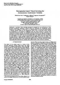
For practical convenience, the upper (2 × 2) submatrix J2×2 of JS must be computed even if the optical markers are not visible. When the instrument is out of the field of view, this sub-matrix is identified in an initial procedure. This identification consists in applying a constant velocity reference (ωx∗ , ωy∗ )t during a short time interval ∆T (see Fig. 8). Should the laser spot positioning performance degrades, it is always possible to start again the identification procedure (see also related work on on-line update of the interaction matrix [12]). For the stability analysis during stage 1, we assume that the organ surface is approximately planar, then d˙ is linearly related to ωx and ωy . In this case, the interaction matrix is reduced to a 2 × 2 matrix : ·
u˙ p v˙ p
¸
= Jω
·
ωx ωy
¸
(25)
and the stability of the visual feedback loop is guarˆω )−1 is positive definite [2]. anteed as long as Jω (J
100 150
200
250
300
350 400 u (pixel)
450
500
550
600
p
Figure 8: Initial on-line identification of matrix Jω (displacements around the image center). and image-based visual servoing along a square using this identification.
mated. During experiments, the orientation of the instrument is controlled by visual servoing in such a way that the laser spot image coordinates reach the desired position p∗ = (u∗p , vp∗ )t and the interaction matrix is provided by the initial identification procedure. Then, the instrument is brought down by a velocity reference vz∗ in open loop, until it is in the field of view. Finally, the depth d0 is controlled (stage 2) to reach the 3-D position (see Figure 10). One can notice the significant perturbations due to the breathing during experiments. up response during visual servoing (pixel) 50
vp response during visual servoing (pixel) 400
0
4
Experiments
200
−50 −100
−200
−200 −250
−400 0
5
10
15
0
5
time (s)
10
15
time (s)
image trajectory during visual servoing (pixel) 500
d0 response during depth servoing (mm) 140 120 100
vp (pixel)
Experiments in real surgical conditions were conducted on living pigs in the operating room of IRCAD. The experimental surgical robotic task consists in positioning the instrument at a 3-D desired position. We use a bi-processor PC computer (1.7 GHz) for image processing and for controlling, via a serial link, a Computer Motion surgical robot. A standard 50 fps PAL endoscopic camera hold by a second robot (at standstill) is linked to a PCI image capture board. For each image, the laser spots barycentre is detected in about 20 ms. Figure 8 shows an image-based visual tracking (a square) experiment with an initial identification procedure (around the image center) realized with the surgical robot-arm and an endo-trainer box. Figure 9 presents some simulations of the proposed imagebased visual servoing and dotted curves represent image trajectories in the case d˙0 cannot be esti-
0
−150
80
0
60 40 20
−500 −250 −200 −150 −100 −50 up (pixel)
0
50
0
5
10
15
time (s)
Figure 9: Image trajectories of laser spot (up , vp ) and d0 responses time during the visual servoing (simulation). Dotted curves correspond to ignoring d˙0 in the first stage (second left member in eq. (22))
up response during visual servoing (pixel) 450
vp response during visual servoing (pixel) 350
[1] A. Casals, J. Amat, D. Prats and E. Laporte. ”Vision Guided Robotic System for Laparoscopic Surgery”. Proc. of the IFAC International Congress on Advanced Robotics. ICAR’95, pp. 33-36, Barcelona, Spain, 1995.
400 350
300 u*p = 384 pixels
300 250
v* = 286 pixels
250
p
200 150
0
10
20
30
200
0
10
20
30
time (s)
time (s)
image trajectory (pixel)
depth d response during visual servoing (mm) 0
350
80
40
p
v (pixel)
300
250 20 initial position 200 100
200
300 up (pixel)
400
500
0
0
20
40 time (s)
60
Figure 10: Image trajectories of laser spot (up , vp ) and d0 responses time during the visual servoing (on living pigs). The effect of breathing is significant.
5
[2] B. Espiau, F. Chaumette, P. Rives, ”A New Approach to Visual Servoing in Robotics”. IEEE Trans. on Robotics and Automation, 8(3), june 1992 [3] M. Hayashibe, Y. Nakamura. ”Laser-pointing endoscope system for intra-operative 3D geometric registration”, Proc. of the 2001 IEEE International Conference on Robotics and Automation. Seoul, Korea, May 2001.
60 desired position
References
Conclusion
In this paper, we present a 3-D positioning system for laparoscopic surgical robots based on visual servoing. In our system, the scene perception is obtained by adding laser pointers and optical markers. To position the surgical instrument, we propose a visual servoing algorithm combining pixels coordinates of laser spots and the estimated distance between organ and instrument. We have shown that these informations are relevant for controlling the 3 dof of a symetrical endoscopic surgical instrument. Successful experiments have been held with a surgical robot on living tissues in a surgical room. For safety reasons, during experiments, we have separated the instrument orientation control from depth control. The proposed technique does not require the knowledge of the initial respective position of the endoscope and the surgical instrument.
Acknowledgements The financial support of the french ministry of research (“ACI jeunes chercheurs” program) is gratefully acknowledged. The experimental part of this work has been made possible thanks to the collaboration of Computer Motion Inc. that has graciously provided the AESOP medical robot. In particular, we would like to thank Dr. Moji Ghodoussi for his technical support. We also thank Prof. Marescaux, Leroy and Soler from IRCAD for their advices, as well as for the use of their facilities.
[4] D.P. Huttenlocher, S. Ullman, ”Recognizing solid objects by alignment with an image”, The International Journal of Computer Vision, 5(2), p.195–212, 1990. [5] S. Hutchinson, G.D. Hager, P.I. Corke, ”A tutorial on visual servo control”, IEEE Trans. on Robotics and Automation, 12(5):p.651–670, October 1996. [6] A. Krupa, C. Doignon, J. Gangloff, M. de Mathelin, L. Soler, G. Morel. ”Towards semi-autonomy in laparoscopic surgery through vision and force feedback control”, Proc. of the Seventh International Symposium on Experimental Robots (ISER), Hawaii, Dec. 2000. [7] A. Krupa, J. Gangloff, M. de Mathelin, C. Doignon, G. Morel, L. Soler, J. Leroy, J. Marescaux. ”Autonomous retrieval and positioning of surgical instruments in robotized laparoscopic surgery using visual servoing and laser pointers”. To appear in the Proc. of the IEEE International Conference on Robotics and Automation, Washington, D.C., May 2002. [8] E Malis, F. Chaumette, S. Boudet, ”2D 1/2 visual servoing”, IEEE Transactions on Robotics and Automation, 15(2), pp.238-250, April 1999. [9] J. Marescaux, J. Leroy and M. Gagner, ”Transatlantic robot-assisted telesurgery” Nature, 413,p.379-380, 2001. [10] P. Martinet, E. Cervera, ”Combining Pixel and Depth Information in Image-Based Visual Servoing”, Proceedings of the 9th International Conference on Advanced Robotics, pp. 445-450, Tokyo, Japan, October 1999. [11] S.J. Maybank. ”The cross-ratio and the j-invariant”, Geometric invariance in computer vision., J. Mundy and A. Zisserman, pp. 107-109, MIT press, 1992. [12] H. Sutanto, R. Sharma, V. Varma Image based Autodocking without Calibration. Proc. of the 1997 IEEE International Conference on Robotics and Automation. Albuquerque, New Mexico, April 1997. [13] G.-Q. Wei, K. Arbter and G. Hirzinger. ”Real-Time Visual Servoing for Laparoscopic Surgery”. IEEE Engineering in Medicine and Biology, 16(1), pp. 40-45, 1997. [14] Y.F. Wang, D.R. Uecker, Y. Wang, ”A new framework for vision-enabled and robotically assisted minimally invasive surgery”, Computerized Medical Imaging and Graphics, vol.22,p.429-437,1998.