contains multiple classes of sensors with different spectral sensitivities .... both cameras, images were obtained with
Image Capture: Modelling and Calibration of Sensor Responses and their Synthesis from Multispectral Images Poorvi L. Vora, Joyce E. Farrell, Jerome D. Tietz, David H. Brainard Computer Peripherals Laboratory HPL-98-187 November, 1998 digital cameras, hyperspectral, multispectral, sensors, simulation, modelling, calibration
This paper describes (a) models for digital cameras, (b) the calibration of the spectral response of a camera and (c) the performance of an image capture simulator. The general model underlying the simulator assumes that the image capture device contains multiple classes of sensors with different spectral sensitivities and that each sensor responds in a known way to light intensity over most of its operating range. The input to the simulator is a set of narrow-band images of the scene taken with a custom-designed hyperspectral camera system [1]. The parameters for the simulator are: the number of sensor classes; the sensor spectral sensitivities; the noise statistics and number of quantization levels for each sensor class; the spatial arrangement of the sensors; and the exposure duration. The output of the simulator is the raw image data that would have been acquired by the simulated image capture device. To test the simulator, we acquired images of the same scene both with the hyperspectral camera [1] and with a calibrated Kodak DCS-200 digital color camera. We used the simulator to predict the DCS-200 output from the hyperspectral data. The agreement between simulated and acquired images validated the image capture response model, the spectral calibrations, and our simulator implementation. We believe the simulator will provide a useful tool for understanding the effect of varying the design parameters of an image capture device.
Internal Accession Date Only
Copyright Hewlett-Packard Company 1998
1 Introduction In this paper we describe, using the Kodak DCS-200 and the DCS-420 as examples, how one can model the sensor response of a camera, calibrate the camera, and then use the model and camera calibration to simulate the camera's response to a scene. The light sensors in many modern image capture devices (e.g. digital scanners and digital cameras) are based on Charge-Coupled Device (CCD) or Active Pixel Sensor (APS) technology. These devices are usually designed so as to have linear intensityresponse functions over most of their operating range [3]. The overall camera system may not exhibit the underlying device linearity, however. For example, there may be a non-linear mapping between the raw sensor output and the digital responses actually available from the camera. Such a non-linearity might be designed into a camera system if the quantization precision of the sensor itself is larger than that of the camera. This is the situation with the Kodak DCS-420. It employs a 12-bit internal data representation for measurements that are linear with respect to light intensity, but its standard control software provides only 8-bits of precision and 8-bit output that is non-linear with respect to light intensity. In this paper we describe methods for testing the camera linearity assumption, as well as a method for determining a static-nonlinearity such as the one used on the Kodak DCS-420. Color cameras require multiple classes of sensors with di�erent spectral sensitivities. By placing color lters in series with either CCD or APS sensors, usually on a pixelby-pixel basis, such multiple classes can be created. When the color lters are placed in a mosaic pattern, one color per pixel, the cameras are referred to as color lter array (CFA) cameras. In this paper we also describe methods for estimating the spectral sensitivity of each class of sensor in a color acquisition device. Evaluation of digital camera design parameters has received considerable attention in the recent literature [4]. These evaluations are based on theoretical models of image statistics and simple image quality metrics. A useful complement to the theoretical approach is to evaluate the performance of di�erent camera designs for actual scenes. A di�culty with this approach is that it is not always feasible. This paper describes a method for constructing, testing and evaluating the performance of an image capture device simulator. A reliable simulator provides a means for evaluating 2
the performance of a complete image capture device design prior to manufacture. The simulator we describe is based on several simplifying assumptions about the image capture device. These are (a) that the optical system is linear and shift invariant, (b) that the response of the sensors to light at varying intensities and wavelengths is known, and (c) that the sensor noise is additive. The input to the simulator is a hyperspectral image of the scene, which provides the full spectral power distribution of the incident light at every image location. These images are acquired with a custom-built hyperspectral camera system [1]. Given the hyperspectral image, the simulator computes the response of the image capture device using the response models developed in this paper. This paper is organised as follows. Section 2 describes the work on camera modelling and section 3 describes the work on camera spectral calibration. In section 4 we describe the simulator and present experimental results verifying its accuracy. Section 5 presents conclusions and future directions.
2 Camera models To test the linearity of the camera response, we measured the intensity-response functions of the Kodak DCS-200 and the Kodak DCS-420 cameras. The DCS-200 contains an 8-bit CCD array while the DCS-420 contains a 12-bit CCD array. For both cameras, images were obtained with a Macintosh host computer using 8-bit drivers provided by Kodak. The camera apertures were kept xed (at f5.6 for the DCS-200 and at f4 for the DCS-420) for all experiments described in this paper. Our basic procedure was to take pictures of a non-selective reference surface (PhotoResearch RS-2 re ectance standard) when it was illuminated by light of di�erent intensities and di�erent wavelengths. We illuminated the surface with light from a tungsten source passed through a grating monochrometer (Bausch & Lomb, 1350 grooves/mm) and varied the intensity by placing neutral density lters in the light path. We used a spectrophotometer (PhotoResearch PR-650) to measure directly the spectrum of the light re ected to the camera. Using this set-up, we measured camera 3
intensity-response functions at several exposure durations for both the DCS-200 and DCS-420 cameras. For each intensity-response series, we assigned an intensity measure of unity to the light reaching the camera when no neutral density lters were in the light path. The intensity of other test lights in the series was de ned relative to the intensity of this light. The relative intensity was determined by nding the scale factor that brought the maximum-intensity spectrum into agreement with the spectrum of the test light. Both the DCS-200 and DCS-420 have a resolution of 1524 � 1012 and the RGB sensors for each camera are arranged in a Bayer mosaic pattern [8]. To obtain sensor data from the camera images we subsampled the camera output using this Bayer pattern. To estimate the mean value of the (dark) additive noise, we acquired images with the lens cap on the camera.
2.1 Linear response model Assuming linearity, the output of a sensor array at grid position (m,n) maybe be approximated as:
r(m; n) � e
N X k=1
s(m; n; k)c(m; n; k)��� + noise 2
(1)
where e is the exposure setting, the argument k represents variation with wavelength, c(m, n, k) is the spectral sensitivity of the sensor at position (m,n), s(m, n, k) is the intensity distribution of light incident on the camera at position (m,n), �� is the wavelength sampling for the intensity and spectral response functions, � is the spatial sampling rate (i.e. the distance between contiguous sensors, assumed to be uniform and identical in both horizontal and vertical directions), and noise represents the sensor measurement noise. Correct calibration allows us to drop the constant �� � in the above sum. In the formulation of equation (1) we neglect optical blur of the camera. This is justi ed for the moment because we consider only images of the Macbeth ColorChecker Chart (MCC), a low spatial frequency target, where optical blurring is not a critical factor. We also assume that the spectral response of a 2
4
single sensor is constant over each pixel and that the wavelength sampling used is ne enough to accurately represent the spectral response. We conducted extensive experiments on the Kodak DCS-200 to check whether its performance is well-described by the linear response model [6]. We measured three intensity-response series, one each at wavelengths of 450, 530, and 600 nm. For each image, we averaged the R, G, B values over a region of 3000 (60 � 50) pixels in the center eld of the camera. For each wavelength, the exposure duration was chosen so that the light energy was roughly within the dynamic range of the camera. The exposure duration was xed for all measurements corresponding to one wavelength. A typical result is shown in Figure 1. The x-axis shows the intensity of the incident light (calculated as described above) and the y-axis shows the camera output value (with the expected value of the noise subtracted). The crosses represent actual data points. The straight lines are t to the data and constrained to pass through the origin. In tting the data, we excluded saturated points and points with very low intensities. The good agreement between the data and the t lines indicate that the DCS-200 has a linear intensity-response function over most of its operating range. RGB values vs. Relative Intensity at 600 nm. 250
Red RGB values minus noise average
200
Green 150
Blue
100
50
0 0
0.1
0.2
0.3
0.4 0.5 0.6 Intensity Measure
0.7
0.8
0.9
1
Figure 1: Typical intensity response, DCS-200 We note that the performance of a second digital camera (the Kodak DCS-420) is not 5
well-described by the linear model, at least when it is operated with the standardlysupplied 8-bit acquistion software [6]. We describe the calibration of the static nonlinearity of the Kodak DCS-420 in the next section.
2.2 Static non-linearity model As shown below, the behavior of the Kodak DCS-420 can be described by a static non-linearity model. For this model, the camera response for a pixel of the ith sensor type pixel is given by
r(m; n) � F (e
N X k=1
s(m; n; k)c(m; n; k)�� � + noise) 2
(2)
where F is a monotonically increasing non-linear function. As an initial test of the DCS-420 linearity, we roughly calculated the average green sensor (G) value at the center of the image eld for a series of images taken under 525 nm illumination. The relationship between intensity and response was clearly non-linear. A probable cause for this non-linearity is the 12-to-8-bit reduction in the image acquisition software. We performed additional measurements at various wavelengths and exposure durations. We extracted the average R, G, and B sensor readings in the center 64 � 64 image region. A typical result is plotted in Figure 2 these measurements were taken under 600 nm illumination and at a 2 sec. exposure setting. In this gure, the expected value of the dark noise has not been subtracted from the camera output. All the results show a similar non-linearity.
2.3 Camera response to variation in exposure To test for linearity with exposure duration in the Kodak DCS-200, we took pictures of the non-selective reference surface under xed illumination at di�erent exposure durations. We did this with narrow band illumination at 470, 530, 570 and 660 nm. Figure 3 shows typical results. As with Figure 1, the crosses represent actual data points with the expected value of the noise subtracted and the lines are ts 6
constrained to pass through the origin. A slight variation from linearity may be due to the fact that the shutter exposure time is not controlled accurately. As the intensity-response function of the DCS-420 is not linear, it would be surprising if its output were linear with exposure duration. We roughly calculated the average green sensor (G) value at the center of the image eld for images of the non-selective reference surface taken at various exposure durations for 525 nm illumination. Figure 4 shows the results with average noise subtracted (x's) overlaid on intensity-response data (replotted as o's). The x-axis represents exposure duration relative to one second and intensity relative to unity. The two readings corresponding to one second and unit intensity are replications of the same illumination condition, so that no scaling of the data were required. The close agreement between the two curves suggests that the same non-linearity mediates both. RGB values vs. Intensity Measure − DCS−420 − 600 nm., 2 sec. 250
RGB values
200
150
100 x: Red
o: Green
50
+: Blue 0 0
0.1
0.2
0.3
0.4 0.5 0.6 Intensity Measure
0.7
0.8
0.9
Figure 2: Typical intensity response, DCS-420
7
1
RGB values vs. Exposure Time at 530 nm. 250
RGB values minus noise average
200
Blue
150 Green Red 100
50
0 0
1
2
3 4 5 Exposure Time in seconds
6
7
8
Figure 3: Response vs. exposure duration, DCS-200
Green Reading vs. Intensity/Exposure Time at 525 nm. 250
Green Reading − Noise Average
200
150
100
50 o: exposure readings x: intensity readings 0 0
0.1
0.2
0.3 0.4 0.5 0.6 0.7 0.8 Intensity Measure/Exposure Time in seconds
0.9
1
Figure 4: DCS-420: Non-linearity with exposure setting 8
2.4 Response model summary 2.4.1 Kodak DCS-200 Our data indicate that the linear response model describes the output of the Kodak DCS-200, at least over the output range 20-240 out of a total range of 0-255 camera units. To obtain the parameters describing a single line for all the data, we t a calibration line to the data for the blue sensor readings of Figure 1, DCS-200 readings for incident illumination at 600 nm and 2 second exposure setting without subtracting out the average dark noise value. The range of numerical values for the data is 24.98 to 222.71. The fractional values arise because camera raw data readings are averaged over an area to obtain these values. The calibration line is the solid line of Figure 5. Measured camera values on a scale of 0-255 are plotted on the x-axis, while linearized fractional output on a scale of 0-1 is plotted on the y-axis. Test of single linear model: DCS−200
Measure of 8−bit (linear) noiseless readings
1
0.8
0.6
0.4
+: Red o: Green
0.2
x: Blue *: Out of linearity range
0
−0.2 0
50
100 150 DCS−200 Reading
200
250
Figure 5: Linearity Map for DCS-200; To verify that the calibration line derived from one intensity response function describes all the data, we can use this line to normalize all of our data and examine it on a single plot. For each measured intensity response function, the intensity measure we used is arbitrary, since we varied both the exposure and wavelength across 9
the di�erent measurements. We can use the calibration line to normalize the data, however. For each data set, we found the highest camera output value in the linear range (below 240) and found its position on the calibration line. We then scaled all the intensity values of that data set by a single normalization scale factor such that the highest camera output value in the linear range would correspond to the intensity factor obtained by looking at the calibration line. This procedure allows us to compare all of our data to the calibration line, Figure 5. The highest camera output value for each data set lies on the line because of the way the normalization is performed. Data points with values below 240 and above 20 all lie close to the line. Data points with values below 20 or above 240 are plotted with asterisks (*) or lie outside the region shown in the plot.
2.4.2 Kodak DCS-420 The Kodak DCS-420 is not linear. To examine whether the static non-linearity response model described its performance, we asked how well a single function F can describe its output across the conditions we measured. We used the intensity-response series measured for the red sensor at 600 nm for a 2 sec exposure (Figure 2) as a reference. This series covered most of the dynamic range of the camera. By interpolating and extrapolating the reference, we obtain a calibration curve for the DCS-420 that maps between sensor values (0 to 256) to intensities that lie between 0 and 1. This intensity measure is in arbitrary units but may be calibrated to physical units. (We used the MATLAB [9] function 'griddata', which implements an inverse distance method, to do the interpolation and extrapolation.) The result is tabulated in Table 1 and graphed as the line in Figure 6. It represents the value of F , (r) , n (or R e ��lh s(�)i(�)d�) of equation (2). 1
10
Table 1: Static Nonlinearity, DCS-420 8-bit
Linearized
8-bit
Linearized
8-bit
Linearized
8-bit
Linearized
8-bit
Linearized
Input
Output
Input
Output
Input
Output
Input
Output
Input
Output
0
0
52
0.0519
103
0.1930
154
0.3820
205
0.6280
1
0
53
0.0541
104
0.1960
155
0.3870
206
0.6330
2
0
54
0.0563
105
0.2000
156
0.3910
207
0.6380
3
0
55
0.0585
106
0.2030
157
0.3960
208
0.6440
4
0
56
0.0607
107
0.2060
158
0.4000
209
0.6490
5
0
57
0.0629
108
0.2090
159
0.4050
210
0.6540
6
0
58
0.0651
109
0.2130
160
0.4100
211
0.6590
7
0
59
0.0674
110
0.2160
161
0.4140
212
0.6650
8
0
60
0.0697
111
0.2190
162
0.4190
213
0.6700
9
0
61
0.0720
112
0.2230
163
0.4240
214
0.6750
10
0
62
0.0743
113
0.2260
164
0.4290
215
0.6810
11
0
63
0.0767
114
0.2300
165
0.4330
216
0.6870
12
0
64
0.0792
115
0.2330
166
0.4380
217
0.6920
13
0
65
0.0816
116
0.2370
167
0.4430
218
0.6980
14
0
66
0.0841
117
0.2400
168
0.4480
219
0.7040
15
0
67
0.0865
118
0.2440
169
0.4520
220
0.7100
16
0
68
0.0890
119
0.2480
170
0.4570
221
0.7160
17
0
69
0.0915
120
0.2510
171
0.4620
222
0.7220
18
0
70
0.0940
121
0.2550
172
0.4670
223
0.7280
19
0.0001
71
0.0965
122
0.2590
173
0.4720
224
0.7340
20
0.0005
72
0.0990
123
0.2630
174
0.4760
225
0.7400
21
0.0009
73
0.1010
124
0.2670
175
0.4810
226
0.7470
22
0.0014
74
0.1040
125
0.2700
176
0.4860
227
0.7540
23
0.0019
75
0.1060
126
0.2740
177
0.4910
228
0.7600
24
0.0025
76
0.1090
127
0.2780
178
0.4960
229
0.7670
25
0.0032
77
0.1120
128
0.2820
179
0.5000
230
0.7750
26
0.0041
78
0.1140
129
0.2860
180
0.5050
231
0.7820
27
0.0050
79
0.1170
130
0.2890
181
0.5100
232
0.7900
28
0.0060
80
0.1200
131
0.2930
182
0.5150
233
0.7970
29
0.0072
81
0.1220
132
0.2970
183
0.5200
234
0.8050
30
0.0086
82
0.1250
133
0.3000
184
0.5250
235
0.8130
31
0.0101
83
0.1280
134
0.3040
185
0.5300
236
0.8220
32
0.0122
84
0.1310
135
0.3080
186
0.5350
237
0.8300
33
0.0148
85
0.1340
136
0.3110
187
0.5400
238
0.8380
34
0.0164
86
0.1370
137
0.3150
188
0.5440
239
0.8470
35
0.0177
87
0.1410
138
0.3180
189
0.5490
240
0.8560
36
0.0195
88
0.1440
139
0.3220
190
0.5540
241
0.8640
37
0.0216
89
0.1470
140
0.3260
191
0.5590
242
0.8730
38
0.0238
90
0.1500
141
0.3290
192
0.5640
243
0.8820
39
0.0260
91
0.1530
142
0.3330
193
0.5690
244
0.8910
40
0.0281
92
0.1570
143
0.3370
194
0.5740
245
0.9000
41
0.0299
93
0.1600
144
0.3410
195
0.5790
246
0.9090
42
0.0314
94
0.1630
145
0.3450
196
0.5840
247
0.9180
43
0.0327
95
0.1670
146
0.3480
197
0.5890
248
0.9270
44
0.0343
96
0.1700
147
0.3520
198
0.5940
249
0.9360
45
0.0363
97
0.1730
148
0.3560
199
0.5990
250
0.9450
46
0.0384
98
0.1770
149
0.3610
200
0.6040
251
0.9550
47
0.0407
99
0.1800
150
0.3650
201
0.6090
252
0.9640
48
0.0430
100
0.1830
151
0.3690
202
0.6130
253
0.9730
49
0.0453
101
0.1870
152
0.3730
203
0.6180
254
0.9830
50
0.0475
102
0.1900
153
0.3780
204
0.6230
255
0.9920
51
0.0497
11
1
Estimate of Noiseless Linearized Sensor Reading
0.9 0.8 0.7 0.6 0.5 0.4 0.3 0.2 0.1 0 0
50
100 150 DCS420 8−bit Value
200
250
Figure 6: Calibration Curve for DCS-420. We tested the accuracy of the calibration curve by asking how well it described the rest of our data. Each set of acquired data points has a di�erent intensity scale. A value of unit intensity corresponds to the maximum intensity for the shutter speed used for that test. To check if the other acquired data points lie on the calibration curve, the intensity values need to be transformed to a single scale. We calculated the scale factor for the conversion for each data set by using the highest measured output value (which corresponds to a unit intensity for that series), nding its position on the calibration curve, and using the fractional intensity value thus obtained as the scale factor. The data points from all of our intensity-response series as well as the exposure data are plotted in Figure 6 along with the calibration curve. The data all lie along the curve.
12
2.5 Variation from Model The data points vary slightly from the linear model for the DCS-200 and from the calibration curve for the DCS-420. In this section, we quantify the variation. To estimate the slight variation from linearity of the DCS-200, we calculated the di�erences between values predicted by the straight line in the linearity plot of Figure 5 and actual values, for measured values above 20 and below 240. These di�erences are plotted in Figure 7. This calculation assigns zero di�erence to the maximum value in each data set because of the way placement of all data points on one curve is performed and is thus only approximate. The error statistics reported below were calculated without using the maximum value in each data set, and are transformed from fractional values from 0-1 to camera values from 0-255. The mean absolute value of the variation is 1.13, and the mean value is 0.58. The average of the noise when estimated from the calibration curve is 12.5. This value is close to the value of 13.6 obtained by directly estimating the dark noise (see section 2.6.1 below). The root mean square value of the variation is 1.45. The maximum error is 4.67 and occurs for a green sensor reading. Noise calculated from intensity and exposure linearity tests 5 x__: Red 4 Noise in camera raw data output units
o−−: Green +....: Blue
3
2
1
0
−1
−2 0
5
10
15 20 Measurement Number
25
30
Figure 7: Variation from linearity - DCS-200 13
35
To quantify the slight variation of the scaled DCS-420 data points from the curve in Figure 6, we calculated the di�erence between the data point and the value on the curve corresponding to the scaled intensity, i.e. the di�erence between indirectly measured values of F , (r) , n and values obtained from the calibration curve. As for the DCS-200, this calculation assigns zero di�erence to the maximum value in each data set and is thus only approximate. The error statistics reported below were calculated without using the maximum value in each data set, and without scaling the linearized output to the camera output scale of 0-255. 1
The average absolute value of the variation was 0.0015. The root mean square value of the variation was 0.0021, approximately 0.5 units per 256 (for comparison with the variation for the DCS-200) and the maximum value was 0.0072, approximately 1.8 units per 256. As can be seen from the plots of Figure 8, the blue has most variation, and the red and green variations are comparable. Noise − non−linearity calibration − DCS420
−3
4
x 10
Noise in fractional intensity units
2
0
−2
−4
x__: Red
o−−: Green
−6
+....: Blue −8 0
5
10
15 20 Measurement Number
25
30
Figure 8: Variation from calibrated curve - DCS-420
14
2.6 Noise Measurements We took a number of dark images at di�erent times during our day-long experiments, and at di�erent exposure durations. We rst discuss the e�ect of exposure duration on dark current noise, and then the e�ect of aging.
2.6.1 Dark current noise as a function of exposure Kodak DCS-200 The dark noise was averaged over the same rectangular area of the center eld as the linearity measurements. The data are tabulated in Table 2. Dark noise shows some variation with exposure duration, up to 4 units, but is quite constant over the di�erent color bands. The mean of the data tabulated is 13.61, 13.63 and 13.61 for red, green, and blue sensors respectively. The overall mean is 13.62. The variances for the three sensor types are 0.78, 0.79 and 0.81 respectively; the corresponding standard deviations are 0.88, 0.89 and 0.90. The overall variance about 13.62 is 0.79 with a standard deviation of 0.89. Variation is greatest for blue sensors and least for red, but the di�erences are slight. The mean values may be compared to those obtained from the variation from linearity calculations in section 2.5. The value of 12.5 obtained there is close to the measured values. The variation values may be compared to the values obtained in section 2.5. The variation from linearity includes the dark noise variation, but is larger because it is not limited to the dark noise variation. It includes other non-linear aspects of the sensor response, including other noise sources like shot noise. Figure 9 illustrates the fact that the variation of dark noise with exposure duration is not monotonic at low exposure durations. This could be because of inaccuracy in the mechanics of the shutter movement. At exposure durations of one-fourth of a second and higher the variation of dark noise with exposure duration is monotonically decreasing. This could be because the e�ects of dark current are averaged out at higher exposure durations.
15
Exposure time in seconds Average Dark Noise Value in Camera Output Units Red Green Blue 8 12.52 12.58 12.51 4 12.85 12.83 12.84 2 12.92 12.93 12.94 1 13.54 13.56 13.51 0.5 13.90 13.92 13.83 0.25 14.27 14.32 14.32 0.125 14.44 14.47 14.45 1/15 14.31 14.32 14.33 1/30 14.54 14.54 14.54 1/60 14.54 14.56 14.60 1/125 11.90 11.88 11.87 Table 2: Dark Noise vs. Exposure Duration, DCS 200.
Dark noise readings vs. Exposure time, logarithmic scale 2.7
x: Red o: Green +: Blue
Logarithm of dark noise readings
2.65
2.6
2.55
2.5
2.45 −5
−4
−3
−2 −1 0 1 Logarithm of exposure time in seconds
2
3
Figure 9: Dark noise vs. exposure duration - DCS-200 16
Kodak DCS-420 The average value of dark current noise is usually subtracted from readings that are known to be linear, i.e. readings predicted by equation (1). As the DCS-420 sensor outputs are the result of a non-linear function operating on the CCD measurements, (equation 2), the dark noise average cannot simply be subtracted from the sensor readings. In fact, our calibration curve (Figure 6) provides an indirect estimate of F , (r) , n and the variability from this curve provides an estimate of the e�ective additive noise. None-the-less, obtaining a direct measure of the dark noise variability seems useful for an estimate of acceptable errors in RGB prediction for camera calibration [7] (see section 3). 1
We took a few dark images (with the lens cap on) at various stages of the experiment, and at various exposure times. We calculated the average value over the same rectangle in the center eld used for other measurements. The average value did not vary much. Its average over the di�erent images was 25.02, 25.01 and 25.06 over red, green and blue sensors respectively. Its overall mean was 25.03. Individual variances about individual means were 0.2375, 0.2207 and 0.2203 for red, green and blue respectively. Its overall variance with respect to the overall mean was 0.2266, and the standard deviation 0.4760. If we convert the dark noise standard deviation to the linear domain (using the average slope of the calibration curve) we get a value of 0.0019. This is a little lower than the measured deviations of the data from the curve. As with the DCS-200, the di�erence is explained by the fact that variation from the calibration curve includes the e�ects of other types of noise besides dark noise.
2.6.2 Dark current noise as a function of aging The data of Table 2 were taken at the end of a day of experiments on the DCS-200, after 120 images were taken with the camera. The next morning, after just a few pictures, a few more dark noise images were taken. The average values of the dark noise images taken over the same rectangular area in the center- eld of the camera are listed in Table 3. 17
The readings for 0.125 seconds are very close to but slightly below those taken earlier. The readings for 1/125 seconds, however, are above those taken earlier by more than 1 unit, an amount which is slightly higher than the standard deviation of the earlier set of readings. Even if this e�ect is real, it is small, and we suspect that treating the camera as a stationary device is satisfactory for most purposes. Table 3: Dark Noise vs. Exposure Duration, DCS 200, Later Readings. Exposure time in seconds Average Dark Noise Value in Camera Output Units Red Green Blue 0.125 14.05 14.04 14.02 1/125 13.08 13.15 13.08
3 Camera calibration In this section, we describe the spectral calibration of the Kodak DCS-200 and Kodak DCS-420 digital cameras. The calibration procedure is based on the response models we developed and tested for these cameras in the previous section [6]. In this section we rst describe how we collected the spectral calibration data. Then we describe simple methods for estimating the camera sensor spectral response functions. Finally, we determine if our estimates of the DCS-200 and DCS-420 can predict the camera responses for images of the Macbeth ColorChecker Chart (MCC).
3.1 Methods For both cameras, we used the 8-bit acquisition software provided by Kodak. In this mode, the response of the DCS-200 is linear with intensity while the response of the DCS-420 is non-linear [6] (see section 2). The camera apertures were kept xed through all the experiments reported here, at f4 for the DCS-420 and f5.6 for the 18
DCS-200. These are the same aperture settings we used to determine the camera response models. To calibrate the camera spectral sensitivities, we measured camera responses to narrow band illumination. We created narrow band stimuli using light from a tungsten source passed through a monochromater (Bausch and Lomb, 1350 grooves/mm) and imaged onto a non-selective re ectance standard (PhotoResearch RS-2). We measured the integrated radiance of each narrow band stimulus using a spectraradiometer (PhotoResearch PR-650). The camera and the radiometer were placed at similar geometric positions with respect to the re ectance standard. It is di�cult to measure the exact spectral power distributions of narrow band sources using the PR-650, since the instrument itself has a bandwidth of 8nm, comparable to that of the narrow band lights. When we performed calculations that required an estimate of the spectral power distributions, we modeled them as narrow gaussians scaled so that they had the same integrated radiance as our measurements. We extracted red, green, and blue (R, G, and B) sensor responses from the camera images and averaged these over a rectangular section in the center of the image (64 � 64 pixels for the DCS-420 and 30 � 25 pixels for the DCS-200). For the DCS-200, we excluded measurements outside of the camera's linear operating range. We corrected the measured responses for the camera dark current by subtracting our estimate of its mean values. For the DCS-420, we used Table 1 to obtain linearized response values. To extend the quantization precision of the cameras, we varied the exposure duration across measurements. We normalized response data across exposure setting by dividing the measured linear response by the exposure duration.
3.2 Simple estimate To perform calculations, we write a version of equation (2) that describes the entire calibration data set. Let r, g, and b be vectors representing the R, G, B readings to a series of narrowband lights. The vectors r, g, and b have Kr , Kg and Kb entries respectively, one for each of the narrowband stimuli used to calibrate the 19
corresponding sensor. Let the full spectrum of the ith narrowband light be si(�), and let the unknown camera spectral sensitivities be cr (�), cg (�) and cb (�). From equation (2) we have,
r=
2 66 6 F (666 64
e(1) Pj cr (�l + j ��)s (�l + j ��)�� 3 7 ... 7 7 P e(i) j cr (�l + j ��)si(�l + j ��)�� 777 + n) ... 7 5 P e(Kr ) j cr (�l + j ��)sKr (�l + j ��)�� 1
(3)
where n is a vector representing measurement noise with variation about the average dark noise value, �� is the wavelength sampling for the radiometric measurements, and e(i) is the exposure setting for the ith measurement. The function F is applied pointwise to each component of the vector it acts on. It is the identity for the DCS200 and the calibrated static non-linearity for the DCS-420. Equations similar to the one above can be written for the readings g and b. The equations for cr (�), cg (�) and cb (�) may be solved in a number of di�erent ways. In the rest of this section and the next we discuss some possibilities. The illumination incident on the camera is narrow-band. Using the ith measurement taken under illumination si centred around �i and ignoring the noise variability, we may estimate the sensor response function cr (�i) as , cr (�i) = e(i) PF s ((r�i)+,j �n��)�� j i i 1
(4)
where ri is the ith component of r, the quantity Pj si(�i + j ��)�� is the integrated radiance of the ith narrowband stimulus and n� is the mean of the noise. For CCD cameras, this mean is typically non-zero. Equation (4) is the `simple' estimate [2]. The function F is the identity for the DCS200 and n� = 13:6 the average measured dark noise value from the experiments detailed in [6] and section 2.6.1. For the DCS-420, the quantity F , (ri) , n� may be obtained from the calibration curve provided in Figure 6. 1
Figures 10 and 11 show plots of the simple estimates obtained for the DCS-200 and for the DCS-420 respectively. The plotted estimates are interpolated from the raw estimates obtained at wavelengths f�ig to a 5 nm wavelength spacing in the range 20
380 nm to 780 nm. In the interpolation procedure, values for wavelengths outside the range where we had data were set to zero. Space limitations prevent us from tabulating the numerical values of the estimate in this report, but they may be found in [7]. The expression X
F (e(i) cr (�j )si(�j )��j + n� )
(5)
was used to calculate RGB values for sensors with the estimated spectral sensitivities. The function F was taken to be the identity for the DCS-200. For the DCS-420, an inverse curve based on the calibration curve of Figure 6 was used. We compared the predicted RGB values to the measurements. Figures 12 and 13 show plots of the measured R, G and B values against the values indicated by expression (5) for the DCS-200 and the DCS-420 respectively. Tables 4 and 5 list the statistics of the estimation errors for the DCS-200 and the DCS-420 respectively.
21
Spectral Response Functions − Kodak DCS−200 − Simple Estimates 9000 8000
Spectral Response Functions
7000 6000 5000 4000 3000
x: Red o: Green +: Blue
2000 1000 0
400
450
500
550 600 Wavelength in nm.
650
700
750
Figure 10: Spectral Response, DCS-200, Simple Estimate Spectral Response Functions − Kodak DCS−420 − Simple Estimates 35
30
Spectral Response Functions
25 x: Red o: Green 20
+: Blue
15
10
5
0
400
450
500
550 600 Wavelength in nm.
650
700
750
Figure 11: Spectral Response, DCS-420, Simple Estimate
22
Measured vs. Predicted values − DCS200 − Simple Estimate 300
250
Predicted values
200
150
100 x: Red o: Green
50
+: Blue 0 0
50
100
150 Measured Values
200
250
300
Figure 12: Measured vs. Predicted Values, DCS-200, Simple Estimate
Measured vs. Predicted values − DCS420 − Simple Estimate 300
250
Predicted values
200
150
100 x: Red o: Green
50
+: Blue 0 0
50
100
150 Measured Values
200
250
300
Figure 13: Measured vs. Predicted Values, DCS-420, Simple Estimate 23
Table 4: Statistics of Estimation Error - DCS-200 - Simple Estimate. RMS value of variation from linearity of DCS-200 is 1.45 [6]. Sensor Mean of Mean of RMS Type Absolute Absolute Error Error % Error Red Green Blue
1.34 0.53 0.50
1.60 1.10 1.29
Camera Maximum Maximum Noise Absolute Absolute Std. Error % Error Deviation 3.68 0.88 16.46 20.27 0.99 0.89 4.09 1.09 0.89 0.90 3.48 9.50
Table 5: Statistics of Estimation Error - DCS-420 - Simple Estimate. RMS value of variation from modelling curve of DCS-420 is 0.50 [6]. Sensor Mean of Mean of RMS Type Absolute Absolute Error Error % Error Red Green Blue
0.83 0.57 0.59
0.88 0.88 0.91
Camera Maximum Maximum Noise Absolute Absolute Std. Error % Error Deviation 1.59 0.49 7.47 6.00 0.74 0.47 1.96 4.17 0.78 0.47 2.36 3.99
24
3.3 Wiener and other estimation methods The Wiener estimate for the spectral sensitivities may be calculated without the assumption that the illuminant sources used to obtain measurements were narrowband. We used a variant of the Wiener estimate that is guaranteed to produce all positive estimates. The Wiener procedure requires that we regard the quantity to be estimated (say x) as a gaussian random variable with known mean and covariance. We took the mean x� to be the simple estimate obtained in the previous section and constructed the covariance matrix �x by assuming that x was the result of a rst-order discrete Gauss-Markov process whose variance was equal to the variance of the entries of x� and whose entryto-entry correlation was equal to the correlation between neighboring entries of x� . We assumed that the entries of n were independently and identically distributed with mean zero and variance equal to 2% of the maximum linearized sensor response (after correction for non-linearity, mean noise level, and exposure duration). We did this for each sensor and obtained results slightly better than those obtained in the previous section. Graphs of the Wiener estimates for the DCS-200 and the DCS-420 are presented in Figures 14 and 15. The spectral response estimates are interpolated as were the simple estimates. Space limitations prevent us from providing the numerical values of the spectral response estimates in this paper, but these values may be found in [7]. Scatter plots of measured values vs. values calculated from the Wiener spectral sensitivity estimates for the DCS-200 and the DCS-420 are plotted in Figures 16 and 17. Tables 6 and 7 list the statistics of the estimation errors for the DCS-200 and the DCS-420 respectively. In contrast to our previous attempts to estimate the spectral sensitivities of the Kodak digital camera [2], the error for both the simple and Wiener estimates are low and close to the rms value predicted by the noise statistics for both cameras. Presumably one factor driving the small error is that we used many narrowband lights to calibrate the sensors. Also, since we used narrowband lights, the simple and the Wiener estimates are very similar. This would not have been so if we had used broadband lights [2], because the simple estimate assumes narrowband lights and is only accurate when this assumption is valid. 25
Non-linear estimation methods like Projections Onto Convex Sets (POCS) [5] are used when the Wiener estimation method gives results that clearly do not satisfy prior knowledge of the solution. For example, POCS would be used if the Wiener estimates gave unreasonable errors in the RGB values. Our estimates satisfy the three known constraints: the set of measured and predicted RGB values agree leaving room for reasonable noise; the lters are reasonably smooth; the lter transmissivities are non-negative. Hence, we did not attempt more complicated non-linear (particularly constrained) estimation methods.
3.4 Veri cation of estimates For the DCS-200, we tested the spectral sensitivity estimates by collecting two images of the MCC under a tungsten illuminant. We compared the actual R, G, and B responses for the 24 color checker patches with values predicted from the spectral sensitivities of the camera and direct radiometric measurements of the light reaching the camera from each patch. To calculate the actual R, G, and B responses we averaged a roughly 20 � 20 pixel region at the center of each patch. The radiometric measurements were taken with the PhotoResearch PR-650 placed at approximately the same position as the camera. Figures 18 and 19 show the predicted vs. measured values for the simple and Wiener estimates respectively. Tables 8 and 9 list the error statistics. It is clear that the estimates are excellent, and perform well on data sets that were not used for the calibration.
26
Spectral Response Functions − Kodak DCS−200 − Wiener Estimates 9000 8000
Spectral Response Functions
7000 6000 5000 4000 x: Red o: Green +: Blue
3000 2000 1000 0
400
450
500
550 600 Wavelength in nm.
650
700
750
Figure 14: Spectral Response, DCS-200, Wiener Estimate Spectral Response Functions − Kodak DCS−420 − Wiener Estimates 35
Spectral Response Functions
30
25
20
15 x: Red o: Green
10
+: Blue 5
0
400
450
500
550 600 Wavelength in nm.
650
700
750
Figure 15: Spectral Response, DCS-420, Wiener Estimate
27
Measured vs. Predicted values − DCS200 − Wiener Estimate 300
250
Predicted values
200
150
100 x: Red o: Green 50
0 0
+: Blue
50
100
150 Measured Values
200
250
300
Figure 16: Measured vs. Predicted Values, DCS-200, Wiener Estimate Measured vs. Predicted values − DCS420 − Wiener Estimate 300
250
Predicted values
200
150
100 x: Red o: Green
50
+: Blue 0 0
50
100
150 Measured Values
200
250
300
Figure 17: Measured vs. Predicted Values, DCS-420, Wiener Estimate
28
Table 6: Statistics of Estimation Error - DCS-200 - Wiener Estimates. RMS value of variation from linearity of DCS-200 is 1.45 [6]. Sensor Mean of Mean of RMS Type Absolute Absolute Error Error % Error Red Green Blue
0.53 0.57 0.28
0.65 0.55 0.62
Camera Maximum Maximum Noise Absolute Absolute Std. Error % Error Deviation 1.42 0.88 8.07 4.22 0.46 0.89 1.34 2.65 0.41 0.90 1.58 4.20
Table 7: Statistics of Estimation Error - DCS-420 - Wiener Estimates. RMS value of variation from modelling curve of DCS-420 is 0.50 [6]. Sensor Mean of Mean of RMS Type Absolute Absolute Error Error % Error Red Green Blue
0.40 0.35 0.47
0.51 0.55 0.66
Camera Maximum Maximum Noise Absolute Absolute Std. Error % Error Deviation 0.62 0.49 2.47 3.69 0.46 0.47 1.34 2.65 0.59 0.47 1.50 2.63
29
Measured vs. Predicted values − MCC − Simple Estimate 300
250
Predicted values
200
150
100
x: Red
50
o: Green +: Blue 0 0
50
100
150 Measured Values
200
250
300
Figure 18: Measured vs. Predicted Values for MCC, DCS-200, Simple Estimate Measured vs. Predicted values − MCC − Wiener Estimate 300
250
Predicted values
200
150
100 x: Red 50
o: Green +: Blue
0 0
50
100
150 Measured Values
200
250
300
Figure 19: Measured vs. Predicted Values for MCC, DCS-200, Wiener Estimate
30
Table 8: Statistics of Estimation Error for MCC - DCS-200 - Simple Estimates. RMS value of variation from linearity of DCS-200 is 1.45 [6]. Sensor Mean of Mean of RMS RMS of Camera Maximum Maximum Type Absolute Absolute Error Variation Noise Absolute Absolute Error % Error in Std. Error % Error Patch Deviation Red 2.76 2.58 3.99 2.08 0.88 14.12 9.72 Green 2.84 2.40 4.25 1.96 0.89 11.78 13.59 Blue 2.74 4.55 3.56 1.83 0.90 10.44 15.53 Table 9: Statistics of Estimation Error for MCC - DCS-200 - Wiener Estimates. RMS value of variation from linearity of DCS-200 is 1.45 [6] Sensor Mean of Mean of RMS RMS of Camera Maximum Maximum Type Absolute Absolute Error Variation Noise Absolute Absolute Error % Error in Std. Error % Error Patch Deviation Red 2.80 2.63 3.97 2.08 0.88 13.63 9.97 Green 2.85 2.41 4.27 1.96 0.89 11.70 13.63 Blue 2.81 4.68 3.60 1.83 0.90 9.95 15.80
31
4 Camera Simulator In sections 2 and 3 we have shown that a linear model with the application of a static non-linearity (if necessary) is exceptionally good at predicting sensor response from digital image sensors. In this section, we describe the use of the linear model to simulate the response of a speci c digital camera to a speci ed scene. The digital camera is de ned by the values of a set of camera design parameters, and the scene is de ned by intensity values as a function of space and wavelength. We also present experimental results that verify the accuracy of the simulator.
4.1 Simulator Description The input to the simulator consists of a set of images which together represent an approximation of the intensity incident on the camera lens as a function of space and wavelength. At present, the input is a set of 31 images taken with the hyperspectral camera system [1]. The 31 images each represent a spatial distribution of the incident intensity over a narrow range of wavelength values. The simulator can also take a di�erent representation of the input, for example a set of images each of which represents the spatial distribution of coe�cients with respect to a basis set of principal components of a database of radiant spectra. In general, the simulator assumes that the intensity distribution as seen by the camera may be written as a weighted sum of a set of images, (s(m; n; k) = PNl cl � Sl (m; n) � pl (k)) where pl (k) represent basis functions for the scene description with respect to wavelength. The simulator uses equation (1) to compute the simulated output image. =1
The parameters of the simulator are: (a) the sensor spectral sensitivities as a function of wavelength, sampled at the same rate as the representation of the input (or represented in terms of the same basis vectors as the input); (b) the exposure time; (c) the noise statistics (mean and variance); (d) the mosaic pattern; (e) the number of bits per pixel of the camera sensors. A nal step of the simulation, not described by equation (1), is to quantize the simulated output to the same number of bits as the simulated device. The output 32
raw data image of the simulator may be directly compared with the camera image for numerical veri cation. For visual quality judgements, we need to demosaic and color correct the outputs of the DCS-200 and the simulator and then compare the color images.
4.2 Simulator veri cation This section describes the experiments performed to verify the accuracy of the simulator for color patches. The DCS-200 was used to take pictures of the MCC in a laboratory illuminated by an incandescent source (Kodak 4400 Slide Projector) at different exposure settings: 1/8, 1/15, 1/30, 1/60 and 1/125 seconds. The hyperspectral camera system was also used to acquire a 31-band hyperspectral image of the same chart under the same conditions. The hyperspectral image, the estimated DCS-200 spectral sensitivities, the exposure durations, the measured noise statistics and the bits per pixel value (8) of the DCS-200 were used to generate simulated images. The simulated images were compared both numerically and visually. Figure 20 is a scatter plot of the real vs. simulated R, G, B values over all the shutter speeds studied in the experiment. It is clear that the agreement between real and simulated values is good. Table 10 lists the numerical error statistics of R, G, and B values averaged over the centre of each patch in both real and simulated images. Since the DCS-200 is an 8-bit camera, the numerical response values range between 0 and 255. The values in the table are computed from response values on this scale. For purposes of comparison, the spatial variation in a dark noise image taken with the DCS-200 has a root mean square value of about 0.89 (see section 2.6.1). Linearity tests for this camera have shown that the root mean square value of the variation from linearity is 1.45 [6] (see section 2.5). Furthermore, the correspondence between predicted and empirical sensor values is consistent across exposure settings, supporting our assumption of linearity with respect to exposure duration - an assumption implicit in equation (1). We visually compared the predicted and empirical sensor data after processing the 33
data with a simple demosaicing routine based on bilinear interpolation. (The complexity of the demosaicing routine is not expected to make a di�erence to visual quality, as the images consist of large color patches.) The real and simulated images have very similar appearances. Simulated vs. Real sensor values for image of MCC
Average value over patch in simulated image
300
250
200
150
100
50
0 0
50
100 150 200 Average value over patch in DCS−200 image
250
300
Figure 20: Scatter plot of MCC colour simulation Table 10: Statistics of Simulation Error for MCC - DCS-200. Exposure Mean of Mean of RMS Error Maximum Maximum Setting Absolute Absolute Absolute Absolute in sec. Error % Error Error % Error 1.49 1.22 2.59 9.07 13.23 3.18 4.03 4.11 9.64 30.99 4.96 7.66 5.43 13.21 24.13 3.47 9.39 3.66 6.75 26.19 1.85 7.22 1.96 3.04 15.16 1 8 1
15 1 30 1 60 1
125
34
5 Conclusions and future directions The use of a linear model with the application of a static non-linearity if necessary is appropriate for the calibration, modelling and simulation of the sensor responses of color lter array cameras. The color delity of output simulated using the linear model is good for a wide range of exposure settings. In the future we will incorporate a model for the optical system to simulate the e�ects of lens blur. The simulation of spatial e�ects (including the e�ect of a lens blur that may vary as a function of position with respect to center- eld and wavelength, inter-sensor charge leakage and the mosaic pattern) on the visual quality of an image will be veri ed by using calibrated hyperspectral input images of scenes with richer spatial variation.
Acknowledgements: This work has been reported in preliminary form in [6, 7, 10, 11]. It was partly supported by a philanthropic grant from Hewlett-Packard to Prof. Brainard.
References [1] D. H. Brainard Hyperspectral Image Data, World Wide Web Site: http://color.psych.ucsb.edu//hyperspectral/, 1997. [2] P. M. Hubel, D. Sherman and J. E. Farrell, A Comparison of Methods of Sensor Spectral Sensitivity Estimation, Proc., IS&T/SID 2nd. Color Imaging Conference: Color Science, Systems and Applications, pp. 45:48, 1994. [3] T. S. Lomheim and L. S. Kalman, Analytical Modeling and Digital Simulation of Scanning Charge-Coupled Device Imaging Systems in Electro-Optical Displays ed. M. A. Karim, Marcel Dekker, 1992. [4] G. Sharma and H. J. Trussell, Figures of merit for color scanners and cameras, IEEE Trans. Image Proc., vol. 6, no. 7, pp. 990-1001, Jul. 1997.
35
[5] H. J. Trussell and M. R. Civanlar, The Feasible Solution in Signal Restoration, IEEE Transactions on Acoustics, Speech, and Signal Processing, Vol ASSP-32, pp 201-212, 1984. [6] P. L. Vora, J. E. Farrell, J. D. Tietz and D. H. Brainard, Digital color cameras 1 - Response models, Hewlett-Packard Company Technical Report, HPL-97-53, March 1997. [7] P. L. Vora, J. E. Farrell, J. D. Tietz and D. H. Brainard, Digital color cameras 2 - Spectral response, Hewlett-Packard Company, Technical Report, HPL-97-54, March 1997. [8] Programmer's Reference Manual Models: DCS200ci, DCS200mi, DCS200c, DCS200m. Eastman Kodak Company, December 1992. [9] MATLAB High-Performance Numeric Computation and Visualization Software, Reference Guide, The MathWorks, Inc., 1992. [10] P. L. Vora, M. L. Harville, J. E. Farrell, J. D. Tietz, D. H. Brainard, `Digital image capture: synthesis of sensor responses from multispectral images', Proceedings, SPIE and IS&T conference on Color Imaging: Device-Independent Color, Color Hard Copy, and Graphic Arts II, 10-14 Feb. 1997, San Jose, California, vol. 3018, pp. 2-11. [11] Poorvi L. Vora, Joyce E. Farrell, Jerome D. Tietz, David H. Brainard, "Linear models for digital cameras", Proceedings, IS&T's 50th Annual Conference, 18-23 May 1997, Cambridge, Massachsetts, pp. 377-382.
36