1: Illustration of the incomplete transform concepts. An additional basis vector (w0) .... learning step is required: this consists in a classification step in which each ...
IMAGE CODING WITH INCOMPLETE TRANSFORM COMPETITION FOR HEVC Adrià Arrufat∗ , Anne-Flore Perrin∗ ∗ Orange
Labs 4, Rue du Clos Courtel 35512 Cesson-Sévigné — FRANCE
ABSTRACT Overcomplete transforms have received considerable attention over the past years. However, they often suffer from a complexity burden. In this paper, a low complexity approach is provided, where an orthonormal basis is complemented with a set of incomplete transforms: those incomplete transforms include a reduced number of basis vectors that allow a reduction on the coding complexity and ensure a certain level of sparsity. The solution has been implemented in the HEVC standard and compression gains of around 1% on average are reported while reducing the decoder complexity in about 5%. Index Terms— Transform coding, orthogonal transforms, sparse data representation, image coding 1. INTRODUCTION Sparse data representation has been an important field of study in the last years thanks to its countless applications in many domains, in which, compression and feature extraction stand out. Sparse representation focuses on finding the most compact representation of a given signal [1]. Amongst them, the K-SVD is one way of designing overcomplete dictionaries to achieve sparse data representation [2]. The usage of multiple complementary transforms to provide sparse representations has been addressed in previous work [3] where the high computational requirements were pointed out: this motivates the work carried out here. In this paper, a low-complexity solution for sparse representation is proposed. The approach is based on a standard orthogonal transform, the discrete cosine transform (DCT), in competition with multiple elementary sparse transforms called Incomplete Transforms. The competition exists in the sense that the encoder selects, for each image block, the transform that provides the best signal representation in the distortion-sparsity plane. The effectiveness of the approach is first measured using a sparsity metric that serves to design effective incomplete transforms based on a learning algorithm. The incomplete transforms are subsequently implemented in High Efficiency
Pierrick Philippe∗† † B-COM
1219, Avenue Champs Blancs 35510 Cesson-Sévigné — FRANCE Video Coding (HEVC), the state-of-the-art image/video coding standard, defined in January 2013 [4]. This paper is organised as follows: section 2 describes the main idea and the motivation to use incomplete transforms. Section 3 proposes a design method for this kind of transforms, which have been implemented HEVC and the results are discussed in section 4. 2. PRINCIPLES OF INCOMPLETE TRANSFORMS In this paper, the concept of incomplete transforms is introduced. They can be considered as a special case of sparse orthonormal transforms [5] in which only one basis vector is retained and considered: consequently, a signal that has been transformed using an incomplete transform has only one coefficient different from zero in the transform domain. In order to be able to represent any signal within a given distortion, incomplete transforms are conceived to work as companions of a main orthogonal transform, such as the DCT for image coding. To illustrate a case where incomplete transforms can be useful, figure 1 presents a two-dimensional scenario, where the small dots symbolise the 2D signals to be transformed. The main transform, whose basis vectors are v0 and v1 , is able to represent the signal in a very efficient way, as v0 follows the main direction of the dark dots. By construction v1 is orthogonal to v0 . However, there exists a secondary direction that cannot be represented compactly using the (v0 , v1 ) basis: both axis are needed to describe their coordinates. Just by adding an extra axis (w0 ) adapted to this secondary direction, an effective and sparser representation of those dots can be achieved. Therefore, the dots plotted in this space can be represented efficiently thanks to the union of two basis. One basis is complete, the second one, which can be conceived as a complete basis, is restricted to only one axis, the principal component: in this way, the compactness is guaranteed as only one transform coefficient need to be transmitted. If only one adapted transform had been used in figure 1 to adapt to all those points, such as the Karhunen-Loève transform (KLT), the main axis would have been placed some-
v1
w0
It is also worth noticing, that those incomplete transforms are non-separable and, therefore, able to exploit any linear correlation amongst pixels within a block. Separable transforms, on the other hand, are only able to exploit correlation of pixels sharing the same row or column. 3. DESIGN OF INCOMPLETE TRANSFORMS
v0
The incomplete transform design is based upon the sparse orthogonal transforms model proposed and detailed in [5]. The original method describes how to derive one optimal transform iteratively for some training data and an initial transform by using a metric that includes a sparsity constraint. In this paper, this method has been further adapted to handle incomplete transforms. 3.1. Incomplete transform learning
Fig. 1: Illustration of the incomplete transform concepts. An additional basis vector (w0 ) is added to assist an orthogonal transform (v0 , v1 ) where in between v0 and w0 , which would not provide sparse representation of the signal. A remarkable consequence of using incomplete transforms is a decrease in complexity when decoding a signal, since there will be one coefficient different from zero, the decoding implies only one basis vector of the incomplete transform multiplied by this coefficient. In image coding, a separable two-dimensional transform writes: �T X = A · A · xT = A · x · AT (1) Assuming the image is composed of 8 × 8 blocks, x stands for the 8 × 8 pixels, and X their frequency representation. A is the 8 × 8 1D transform. The usual transform used in image coding is the DCT, whose fast algorithm requires 12 multiplications and 29 additions per 8 × 1 vector. As 8 vectors per block need to be processed both for the vertical and horizontal transform, processing an 8 × 8 block requires a total of 192 multiplications and 464 additions. This number of operations is identical for the inverse transform. For an incomplete transform, only one axis needs to be processed: each axis being formed by 64 values in this example. Consequently, only 64 multiplications and 63 additions are need to transform the input block x into the transform domain. For the inverse transformation, only 64 multiplications are needed. As a result, in this case, the incomplete transforms can be applied with an number of operations of approximatively one third of the cost of regular separable transforms. This complexity reduction benefits both the encoder and the decoder.
The method proposes a weighted rate-distortion metric that is able to provide different trade-offs. This metric includes a measure of the distortion in the mean square error sense of the quantised samples and a sparsity constraint, as explained below. � � 2 Aopt = arg min ∑ min kxi − AT ci k2 + λ kci k0 (2) A
∀i
ci
Where xi is signal from the training set, e.g. a block of pixels reshaped into a N 2 × 1 vector, Xi = A · xi are the transformed coefficients using the transform A and ci are the quantised transformed coefficients. AT is the inverse transform, since A is chosen orthonormal. The constraint in the cost function is the `0 norm of the coefficients, i.e. the number of non-zero coefficients, also called the number of significant coefficients. Finally, λ is the Lagrange multiplier. The equation 2 is minimised in two steps. First, the optimal coefficients are obtained by hard-thresholding Xi . Afterwards, the transform is updated given the hard-thresholded coefficients ci and the xi . A detailed resolution of this equation is described in [5], as well as the relation between λ and the hard-thresholding parameter. The algorithm iterates over the two steps until the metric converges. The design of an incomplete transform takes one extra step: one and only one coefficient is kept after hardthresholding, the first one. Consequently, only X0 is considered and the level of sparsity is guaranteed as kci k0 = 1. This makes the incomplete transform to have only one meaningful basis vector. Therefore, for a given set of training signals, one obtains a transform consisting of one meaningful basis vector. The remaining vectors, albeit constituting a basis, are useless for the aim of the paper.
3.2. Multiple incomplete transforms Since incomplete transforms are designed with a strong sparsity constraint of the quantised coefficients, it seems reasonable to generate several incomplete transforms to be able to adapt to different signal natures. However, an incomplete transform cannot represent accurately a signal provided a desired level of fidelity (e.g. a distortion criterion). Consequently, the purpose of this paper is to complement a set of incomplete transforms with a standard orthogonal transform, such as the DCT. As a result, a coding scheme based on such an approach is able to compress a signal at any quality level and might be able to be efficient sparsity-wise thanks to the incomplete transforms. A learning algorithm and classification algorithm based on the metric defined in equation 2 has been implemented to design a set of 1 + N transforms: N incomplete transforms that complement a standard orthogonal transform, the DCT. In order to design multiple transforms, an additional learning step is required: this consists in a classification step in which each learning signal is assigned to the transform, complete or incomplete, that provides the best representation in a rate distortion sense. The rate distortion metric is consistent with the one defined in equation 2 and its purpose is to assign a signal xi to the transform An that minimises the value: 2
δn = kxi − ATn ci,n k2 + λ kci,n k0
input : A training set of image signals x output: Set of N incomplete transforms An Initial random classification into 1 + N classes while !convergence do for n = 1 to N do Learn an inc. tr. on Classn using equation 2 end foreach block x do for n = 0 to N do 2 δn = kx − ATn ck + λ kck0 end n∗ = arg min(δn ) n
Classn∗ .append(x) end end Algorithm 1: Multiple incomplete transform design
100 % 90 % 80 % 70 % 60 %
(3)
0
4
8
16
32
number of incomplete transforms
To this end, the representation of any signal xi is computed for all transforms An , delivering a set of Xi,n , subsequently quantised into ci,n . The quantisation operator is the hardthresholding function presented before, but only the first frequency coefficient is retained for the incomplete transforms. Therefore, the sparsity constraint, i.e. the second half of equation 3 equals to λ for the incomplete transforms and proportional to the number of significant coefficients for the DCT. Once the learning signals have been classified given a set of transforms, each incomplete transform is updated using the learning algorithm of section 3. The classification/transform update steps are repeated until convergence. Note that only transforms A1 to AN are updated while A0 (the DCT) is also considered in the classification step. To illustrate the effectiveness of the algorithm, figure 2 presents how the increase of the number of incomplete transforms is able to provide a more sparse representation of the signal. To evaluate this, the average number significant coefficients is computed at a similar distortion level for different coding configurations (from 1 to 32 incomplete transforms used in conjunction with the DCT). The results are presented relative to the reference system which consists of a coding system using the DCT alone, such as HEVC. As the number of incomplete transforms is increased, the proportion of significant coefficients is decreased to 66% of
Fig. 2: Percentage of non-zero coefficients referred to the DCT its original value: this validates the fact that more sparse representations can be achieved with the adjunction of incomplete transforms to the traditional DCT transform. The result of a learning experiment is shown in figure 3, where 32 8 × 8 incomplete transforms are presented. For each one, only the first basis vector is displayed, since is the only one delivering significant frequency coefficients. In the case of two-dimensional signals, like images, incomplete transforms can be directly interpreted as texture patterns. The learning set in this experiment is made of prediction residuals extracted from a directional mode from the HEVC coding scheme. The selected mode (intra prediction 6) is an angular prediction of approximatively +26◦ . Accordingly, the blocks selected by HEVC for this mode mostly present a directional pattern following that direction. It can be observed how the incomplete transforms have patterns containing that particular direction, each exhibiting a particular band-shaped pattern. Note that the DCT requires a significant number of coefficients to represent such directional, and inherently non-separable, patterns.
Class A (2560 × 1600)
Class B (1920 × 1080) Fig. 3: List of 32 incomplete transforms for 8 × 8 blocks 4. APPLICATION TO IMAGE CODING The usefulness of incomplete transforms has also been applied to a practical environment, more precisely, inside the HEVC, the latest video coding standard, which is considered as the most performing image coder as of today [6]. To evaluate the coding performance of the approach, a set of incomplete 8 × 8 transforms is designed for each HEVC intra prediction mode. At the encoder, for each block, the best prediction mode/transform pair is selected. The conventional HEVC work flow is used except for two changes: 1. The signalling of the selected transform is requested. A flag + index approach has been retained here for its simplicity. If the DCT is selected, 0 is signalled, otherwise a flag is set to 1 and a fixed-length codeword indicates the incomplete transform index. 2. As the incomplete transforms retain only the first coefficient, the position of the last significant coefficient does not need to be conveyed. Experiments have been performed following the common test conditions described in [7] for an established test set (independent from our learning set). Sequences have been coded in all intra (AI) mode, meaning that each image is coded independently. As specified in the test conditions, the improvement are presented as percentage of bit rate reduction relative to the HEVC coding scheme, using the Bjøntegaard Distortion-rate (BD-rate) metric [8]. Table 1 shows that around 1% of bit-rate reduction with regards to the HEVC standard can be achieved using this technique. There are some sequences which present notable gains over HEVC, such as SteamLocomotiveTrain and BasketballDrill. This is due to the large amount of diagonal patterns in those sequences, which are hardly handled by separable transforms like the DCT. Complexity-wise, the proposed system is much more attractive that the previous one from [3], where regular nonseparable transforms are tested in the HEVC rate-distortion optimisation loop, which lead to a complexity of around 8
Class C (832 × 480)
Class D (416 × 240) Class E (1280 × 720)
Sequence PeopleOnStreet Traffic NebutaFestival SteamLocomotiveTrain BasketballDrive BQTerrace Cactus Kimono1 ParkScene BasketballDrill BQMall PartyScene RaceHorses BasketballPass BQSquare BlowingBubbles RaceHorses FourPeople Johnny KristenAndSara Average
Y BD-rate -0.64% -0.68% -0.91% -5.25% -0.99% -1.06% -1.38% -0.31% -0.15% -6.22% -0.66% -0.18% -0.44% -0.47% -0.25% -0.21% -0.32% -1.07% -1.25% -1.15% -1.18%
Table 1: BD-rate savings referred to HEVC times the one from HEVC [3]. Using incomplete transforms leads to a complexity 2.7 times higher than that of HEVC. On the decoder side, complexity has been decreased due to the reduction in the number of operations with regards to the DCT when using incomplete transforms. Whilst the previous system increased the decoding complexity by 30% [3], the incomplete transforms reduce the decoding time in 5% on average. Keeping in mind that the transform does not represent the whole decoding process and that the DCT is still used, complexity reductions affecting the transform are moderate. 5. CONCLUSIONS This paper has proved the effectiveness of incomplete transforms. When used as complementary transforms, they are able to increment the sparsity of the signal in the transform domain. The number of non-zero coefficients has been reduced to around two thirds of its original value. First experimental results on the HEVC-based image coder prove that incomplete transforms can be used to obtain some compression gains, 1% on average and up to 6% bit-rate reduction is achieved, with a slight decrease of the decoding complexity.
6. REFERENCES [1] Ke Huang and S. Aviyente, “Sparse representation for signal classification,” in In Adv. NIPS, 2006. [2] M. Aharon, M. Elad, and A. Bruckstein, “K-SVD: An algorithm for designing overcomplete dictionaries for sparse representation,” Signal Processing, IEEE Transactions on, vol. 54, no. 11, pp. 4311–4322, Nov 2006. [3] A. Arrufat, P. Philippe, and O. Déforges, “Ratedistortion optimised transform competition for intra coding in HEVC,” in Visual Communications and Image Processing, 2014. IEEE Proceedings on, 2014, pp. 73–76. [4] G.J. Sullivan, J. Ohm, Woo-Jin Han, and T. Wiegand, “Overview of the High Efficiency Video Coding standard,” Circuits and Systems for Video Technology, IEEE Transactions on, vol. 22, no. 12, pp. 1649–1668, 2012. [5] O.G. Sezer, O. Harmanci, and O.G. Guleryuz, “Sparse orthonormal transforms for image compression,” in Image Processing, 2008. ICIP 2008. 15th IEEE International Conference on, 2008, pp. 149–152. [6] P. Hanhart, P. Korshunov, and T. Ebrahimi, “Subjective Evaluation of Higher Dynamic Range Video,” in SPIE Optical Engineering + Applications, 2014, Applications of Digital Image Processing. [7] F. Bossen, “Common test conditions and software reference configurations,” Tech. Rep. JCTVC-I1100, ITU-T, Geneva, Switzerland, May 2012. [8] G. Bjøntegaard, “Calculation of average PSNR differences between RD-curves,” Tech. Rep. VCEG-M33, ITU-T, Austin, Texas, April 2001.