2254
IEEE TRANSACTIONS ON IMAGE PROCESSING, VOL. 19, NO. 9, SEPTEMBER 2010
Image Segmentation by MAP-ML Estimations Shifeng Chen, Liangliang Cao, Yueming Wang, Jianzhuang Liu, Senior Member, IEEE, and Xiaoou Tang, Fellow, IEEE
Abstract—Image segmentation plays an important role in computer vision and image analysis. In this paper, image segmentation is formulated as a labeling problem under a probability maximization framework. To estimate the label configuration, an iterative optimization scheme is proposed to alternately carry out the maximum a posteriori (MAP) estimation and the maximum likelihood (ML) estimation. The MAP estimation problem is modeled with Markov random fields (MRFs) and a graph cut algorithm is used to find the solution to the MAP estimation. The ML estimation is achieved by computing the means of region features in a Gaussian model. Our algorithm can automatically segment an image into regions with relevant textures or colors without the need to know the number of regions in advance. Its results match image edges very well and are consistent with human perception. Comparing to six state-of-the-art algorithms, extensive experiments have shown that our algorithm performs the best. Index Terms—Graph cuts, image segmentation, Markov random fields, maximum a posteriori, maximum likelihood.
I. INTRODUCTION
T
HE problem of image segmentation and visual grouping has received extensive attention since the early years of computer vision research. It has been known that visual grouping plays an important role in human visual perception. Many computer vision problems, such as stereo vision, motion estimation, image retrieval, and object recognition, can be solved better with reliable results of image segmentation. For example, results of stereo vision based upon image segmentation are more stable than pixel-based results [1]. Although the problem of image segmentation has been studied for more than three decades, great challenges still remain in this research. Manuscript received July 15, 2008; revised February 16, 2010. First published April 01, 2010; current version published August 18, 2010. This work was supported in part by the Natural Science Foundation of China under Grants No. 60903117 and No. 60975029, in part by the Shenzhen Bureau of Science Technology & Information, China under Grant No. JC200903180635A, and in part by the the Research Grants Council of the Hong Kong SAR, China under Project No. CUHK 415408. The associate editor coordinating the review of this manuscript and approving it for publication was Dr. Ilya Pollak. S. Chen is with the Shenzhen Institutes of Advanced Technology, Chinese Academy of Sciences, Shenzhen 518055 China (e-mail:
[email protected]. cn). L. Cao is with the Department of Electrical and Computer Engineering, University of Illinois at Urbana-Champaign, Urbana-Champaign, Urbana, IL 61801 USA (e-mail:
[email protected]). Y. Wang is with the Department of Information Engineering, The Chinese University of Hong Kong, Hong Kong, and also with the College of Computer Science, Zhejiang University, Hangzhou 310027 China (e-mail: ymwang@ie. cuhk.edu.hk). J. Liu and X. Tang are with the Department of Information Engineering, The Chinese University of Hong Kong, Hong Kong, and also with the Shenzhen Institutes of Advanced Technology, Chinese Academy of Sciences, Shenzhen 518055 China (e-mail:
[email protected];
[email protected]). Color versions of one or more of the figures in this paper are available online at http://ieeexplore.ieee.org. Digital Object Identifier 10.1109/TIP.2010.2047164
A. Related Work Available image segmentation algorithms can be classified into two groups: contour-based approaches and region-based approaches. Contour-based approaches try to find the boundaries of objects in an image, while region-based approaches attempt to split an image into connected regions. The main idea of contour-based approaches is to start with some initial boundary shape represented in the form of a spline curve, and iteratively modify it by shrink and expansion operations to minimize some energy function. These approaches are physics-based models that deform under the laws of Newton mechanics, in particular, by the theory of elasticity expressed in the Lagrange dynamics. Many contour-based segmentation algorithms [2]–[9] have been developed in the past two decades. One problem existing in these algorithms is that they are easy to get trapped in local minima. In addition, they need manually specified initial curves close to the objects of interest. Region-based approaches try to classify an image into multiple consistent regions or classes. Thresholding is the simplest segmentation method but its performance is usually far from satisfactory. Watershed segmentation [10], [11] is one of the traditional region-based approaches. The watershed transform is often used to segment touching objects. It finds intensity valleys in an image if the image is viewed as a surface with mountains (high intensity regions) and valleys (low intensity regions). Morphological operations are always used to handle the over-segmented problem in the output obtained by the watershed transform. Usually, watershed is used for the segmentation of foreground and background (two-class) of an image. For a general color image with many different regions, it often gives a bad result. It is also sensitive to the morphological structuring element. Another kind of approaches to region-based segmentation is finding compact clusters in a feature space [12]–[15]. The -means algorithm [12] is the basic one. However, the -means is not good enough because it does not take account of the spatial proximity of pixels. It is, thus, often used in the initialization step for other approaches. Expectation-maximization (EM) [13] performs segmentation by finding a Gaussian mixture model in an image feature space. One shortcoming of EM is that the number of regions is kept unchanged during the segmentation, which often causes wrong results because different images usually have different numbers of regions. Theoretically, the minimum description length (MDL) principle [13] can be used to alleviate this problem, but the segmentation has to be carried out many times with different region numbers to find the best result. This takes a large amount of computation, and the theoretically best result may not accord with our perception. In [14] and [15], a mean shift algorithm is proposed for image segmentation. Mean shift is a nonparametric clustering technique which neither requires to know the number of
1057-7149/$26.00 © 2010 IEEE
CHEN et al.: IMAGE SEGMENTATION BY MAP-ML ESTIMATIONS
2255
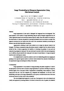
number of clusters is given in the beginning and cannot be adjusted during the segmentation. Besides, the segmentation result is sensitive to this number, as pointed out by the authors. Recently, some researchers paid attention to learning-based segmentation of objects of a particular class from images [28]–[31]. Different from common segmentation methods, this work requires to learn the parameters of a model expressing the same objects (say, horse) from a set of images. These techniques can generate impressive segmentation results for specific objects, but they cannot be used for general image segmentation and for object extraction without the priors learnt. B. Outline of Our Work Fig. 1. (a) Original color image. (b)–(d) Three components of (a) in L*a*b* color space. (e) Texture contrast of (a).
clusters in advance nor constrains the shapes of the clusters. However, it often obtains over-segmented results for many natural images. In [16] the distribution of texture features are modeled using a mixture of Gaussian functions. Unlike most existing clustering methods, it allows the mixture components to be degenerate or nearly-degenerate. A simple agglomerative clustering algorithm derived from a lossy data compression approach is used to segment such a mixture distribution. Recently, a number of graph-based approaches are developed for image segmentation. Shi and Malik’s [17] and Yu and Shi’s [18] normalized cuts are able to capture intuitively salient parts in an image. The normalized cut criterion is a significant advance over the previous work in [19] with a min cut criterion, which tends to find too small components. Normalized cuts are a landmark in current popular spectral clustering research, but it is not perfectly fit to the nature of image segmentation because ad hoc approximations must be introduced to relax the NP-hard computational problem. These approximations are not well understood and often lead to unsatisfactory results. In addition, the heave computational cost is a disadvantage rooted in spectral clustering algorithms. In [20], an efficient graph-based image segmentation algorithm is developed, but the over-segmentation problem remains in its results. Tu and Zhu [21] presented a generative segmentation method under the framework of maximum a posteriori (MAP) estimation of Markov random fields (MRFs), with the Markov Chain Monte Carlo (MCMC) used to solve the MAP-MRF estimation. This method suffers from the computation burden. In addition, the generative approach explicitly models regions in images with many constraints, resulting in the difficulty of choosing parameters to express objects in images. Segmentation by generalized Swendsen-Wang cuts [22] is a faster method than that in [21]. The two methods produce similar results as they share the same underlying model. Another popular segmentation approach based upon MRFs is graph cut algorithms [23]–[26]. These algorithms rely on human interaction, and solve the twoclass segmentation problem only, i.e., separating an image into only background and object regions, with some manually given seed points. In [27], Zabih and Kolmogorov used graph cuts to obtain the segmentation of multiple regions in an image, but the
This paper1 proposes a new image segmentation algorithm based upon a probability maximization model. An iterative optimization scheme alternately making the MAP and the maximum likelihood (ML) estimations is the key to the segmentation. We model the MAP estimation with MRFs and solve the MAP-MRF estimation problem using graph cuts. The result of the ML estimation depends upon what statistical model we use. Under the Gaussian model, it is obtained by finding the means of the region features. It is shown that other statistical models can also fit in our framework. The main contributions of this work include: 1) a novel probabilistic model and an iterative optimization scheme for image segmentation, and 2) using graph cuts to solve the multiple region segmentation problem with the number of regions automatically adjusted according to the properties of the regions. Our algorithm can cluster relevant regions in an image well, with the segmentation boundaries matching the region edges. Extensive experiments show that our algorithm can obtain results highly consistent with human perception. The qualitative and quantitative comparisons demonstrate that our algorithm outperforms six other state-of-the-art image segmentation algorithms. The rest of this paper is organized as follows. In Section II, we build the framework of our probabilistic model for image segmentation. Section III discusses the detail of our algorithm with its convergency proof. Extensive experimental results are given in Section IV to show the performance of our algorithm. Section V concludes the paper. II. NEW PROBABILISTIC MODEL In this section, we first introduce the features used to describe the properties of each pixel, and then present the new probabilistic model. For a given image , the features of every pixel are expressed by a 4-D vector (1) , , and are the components of in the where denotes the texture feature of L*a*b* color space, and . Several classical texture descriptors have been developed in [13], [33], [34], and [35]. In this paper, the texture contrast deto ) is chosen as the texfined in [13] (scaled from ture descriptor. Fig. 1 shows an example of the features. 1The
preliminary version of this paper was presented in CVPR 2007 [32].
2256
IEEE TRANSACTIONS ON IMAGE PROCESSING, VOL. 19, NO. 9, SEPTEMBER 2010
The task of image segmentation is to group the pixels of an image into relevant regions. If we formulate it as a labeling problem, the objective is then to find a label configuration where is the label of pixel denoting which region this pixel is grouped into. Generally speaking, a “good” segmentation means that the pixels within a region should share that does not homogeneous features represented by a vector change rapidly except on the region boundaries. The introducallows the description of a region, with which high tion of level knowledge or learned information can be incorporated into the segmentation. Suppose that we have possible region labels. A 4-D vector
Assuming that the observation of the image follows an indeas pendent identical distribution (i.i.d.), we define
(7) where is the data penalty function which imposes for given . The data the penalty of a pixel with a label penalty function is defined as
(2) is used to describe the properties of label (region) , where the have the similar meanings to those of four components of and will be derived the corresponding four components of in Section II-B. be the union of the region features. If Let and are known, the segmentation is to find an optimal label configuration , which maximizes the posterior possibility of the label configuration (3) where can be obtained by either a learning process or an initialized estimation. However, due to the existence of noise and diverse objects in different images, it is difficult to obtain that is precise enough. Our strategy here is to refine according to the current label configuration found by (3). Thus, we propose to use an iterative method to solve the segmentation problem. and are the estimation results in the th Suppose that iteration. Then the iterative formulas for optimization are defined as
(8) We restrict our attention to MRF’s whose clique potentials involve pairs of neighboring pixels. Thus (9)
where is the neighborhood2 of pixel . , called the smoothness penalty function, is a clique potential function, which describes the prior probability of a particular . We label configuration with the elements of the clique define the smoothness penalty function as follows using a generalized Potts model [36]:
(4) (10) (5) This iterative optimization is preferred because (4) can be solved by the MAP estimation, and (5) by the ML estimation. Based upon this framework, next we will explain how the MAP and ML estimations are implemented. A. MAP Estimation of
From
Given an image and the potential region features , we infer by the Bayesian law, i.e., can be obtained by
(6) which is a MAP estimation problem and can be modelled using MRFs.
where , called brightness contrast, is a denotes how different the brightnesses of and are, is used to control the contribution of smoothness factor, to the penalty, and is 1 if its argument is true and 0 otherwise. From our experiments, we found that is a good choice, where denotes the expectation of all the depicts two kinds pairs of neighbors in an image. of constraints. The first enforces the spatial smoothness; if two neighboring pixels are labeled differently, a penalty is imposed. The second considers a possible edge between and ; if two neighboring pixels cause a larger , then they have greater likelihood to be partitioned into two regions. Fig. 2 is an example of the brightness contrast. In our algorithm, the boundaries of the segmentation result are pulled to match the darker pixels in Fig. 2(b) and (c), which are more likely to be edge pixels. 2In this paper, the neighborhood of pixel p consists of the two horizontal and two vertical neighbors of p.
CHEN et al.: IMAGE SEGMENTATION BY MAP-ML ESTIMATIONS
2257
lead to different eswhere different formulations of timations of . For our formulation in (8), it follows that: (18)
Fig. 2. Example of the brightness contrast. (a) The original image. (b) The brightness contrast in the horizontal direction. (c) The brightness contrast in the vertical direction.
Therefore, (17) can be written as for each From (19), we obtain the ML estimation
From (6), (7), and (9), we have
(19)
, where (20)
(11)
Taking the logarithm of (11), we have the following energy function:
with being the number of pixels within region . Here (20) , , , and in is exactly the equation to obtain (2). is unNote that when the label configuration known, finding the solution of (17) is carried out by clustering the pixels into groups. In this case, the ML estimation is achieved by the -means algorithm [12], which serves as the initialization in our algorithm described in Section III.
(12) C. Non-Gaussian Modeling . It includes two parts: the
where data term
(13) and the smoothness term
The definition of in (8) uses the Gaussian model to describe a uniform region. Some other distributions in the modeling of natural images, such as the exponential family distributions [37], [38], can also be used in our framework. Let us take another popular model, the Laplace model [39], as an example. To replace the Gaussian model with the Laplace model, we modify (7) as
(14)
From (12), we see that maximizing is equivalent for a given . In this to minimizing the Markov energy paper, we use a graph cut algorithm to solve this minimization problem, which is described in Section III. B. ML Estimation of
From
If the label configuration is given, the optimal should , or minimize equivalently. maximize Thus, we have (15) or (16) where denotes the gradient operator. Since independent of , we obtain
is
(17)
(21) where the data penalty is defined as (22) With this data penalty, the MAP estimation is the same as when the Gaussian model is used. However, the ML estimation result is different from (20) and becomes (23) denotes the median of the elements in a set where [40]. In addition to the above parametric models, we can also use nonparametric distributions to describe the region features. Similar to the parametric models, the data penalty functions are defined as the negative logarithm of different likelihood functions in different nonparametric models (e.g., a histogram clustering model is used in [41]). In summary, different statistical models lead to different definitions of the data penalty. Given different data penalties, the MAP estimations are the same, but the ML estimation results
2258
IEEE TRANSACTIONS ON IMAGE PROCESSING, VOL. 19, NO. 9, SEPTEMBER 2010
Fig. 3. Relabeling of the regions. (a) Result before the relabeling. (b) Result after the relabeling.
depend upon the used models. In the rest of this paper, we only consider the Gaussian model. III. PROPOSED ALGORITHM We first give the description of the algorithm for image segmentation, and then prove its convergence. Algorithm Description defined in (12), the estimations of With (4) and (5) are now transformed to
and
Fig. 4. Segmentation example. (a) Original image. (b) Result of initial -means clustering with . (c) Result of the first iteration with adjusted to 8 automatically. (d) Converged result after 4 iterations with changed to 6 automatically.
K
K = 10
K K
in
(24) (25) The two equations correspond to the MAP estimation and the ML estimation, respectively. The algorithm to obtain and is described as follows. Algorithm: Image Segmentation: Input: an RGB color image. Step 1: Convert the image into L*a*b* space and calculate the texture contrast. Step 2: Use the -means algorithm to initialize . Step 3: Iterative optimization. 3.1: MAP estimation—Estimate the label conbased upon current using the figuration graph cut algorithm [36]. 3.2: Relabeling—Set a unique label to each connecting region to form a new cluster, obtaining a new . 3.3: ML estimation—Refine based upon current with (20). Step 4: If and do not change between two successive iterations or the maximum number of iterations is reached, go to the output step; otherwise, go to step 3. Output: Multiple segmented regions of the image. We explain step 3.2 in more details here. After step 3.1, it is possible that two nonadjacent regions are given the same label. For example, the upper-left and the lower-right regions in Fig. 3(a) are both labeled by 1. After step 3.2, each of the connected regions has a unique label [see Fig. 3(b)]. The MAP estimation is an NP-hard problem. Boykov et al. [36] proposed to obtain an approximate solution via finding the minimum cuts in a graph model. Minimum cuts can be obtained by computing the maximum flow between the terminals
of the graph. In [36], an efficient max-flow algorithm is given for solving the binary labeling problem. In addition, an algorithm, called expansion with the max-flow algorithm embedded, is presented to carry out multiple labeling iteratively. In our algorithm, the expansion algorithm is used to perform step 3.1. Besides the graph cuts, other techniques such as belief propagation can also be used to solve the MAP-MRF problem. A comparative study can be found in [42]. One remarkable property of our algorithm is the ability to adjust the region number automatically during the iterative optimization with the relabeling step embedded into the MAP and ML estimations. Fig. 4 gives an example to show how the iterations improve the segmentation results. Comparing Fig. 4(b)–(d), we can see that the final result is the best. Another property of our algorithm is that it is insensitive to the value of in the initialization step with the -means algorithm. From Figs. 4 and 5 we can see that the converged results with , 10, and 20 are very close. Now we analyze the computational complexity of the algotime rithm. In step 2, the -means algorithm takes is the number of pixels in an image, is the [12], where is the number of features used to represent a pixel/region, number of clusters, and is the number of iterations. In our , is set to 10, and is set to 100. Both application, time. In step 3, the main comstep 3.2 and step 3.3 take putational burden is the use of the graph cut algorithm (the expansion) in step 3.1. The max-flow algorithm is linear in practime tice [36]. The expansion algorithm takes to carry out the MAP estimation during the -th execution of is the number of label candidates and step 3.1, where is the number of iterations inside the expansion. Let be the number of executions of step 3.1. Then the computational com. plexity of our algorithm is In general, ranges from 1 to 50, is less than 5, and is less than 10. Using a PC with Pentium 2.4 G CPU and 2 G RAM, our algorithm takes less than 2 minutes to handle a 321 481 image.
CHEN et al.: IMAGE SEGMENTATION BY MAP-ML ESTIMATIONS
K
2259
K
Fig. 5. Segmentation results with different values in the initial -means. The original image is shown in Fig. 4(a). (a) Result of initial -means clustering . (b) Converged result of (a). (c) Result of initial -means clustering with . (d) Converged result of (c). with
K=5 K = 20
K K
Algorithm Convergence We prove that the proposed algorithm is convergent in this , section. Suppose that after the th iteration, the energy is the configuration is , and the union of region features is . The MAP estimation is to estimate the configuration by minimizing the energy. Therefore, after the MAP estimation step of the th iteration, the energy decreases or keeps unchanged, i.e.,
Fig. 6. Segmentation results on the “landscape” images.
(26) Suppose that the configuration is after the relabeling step. This step only changes the labels of some regions but not their features, i.e., for each pixel (27) Therefore, from (8) and (13), the relabeling step does not change the data term. On the other hand, after the relabeling, for two neighboring pixels and , it is easy to see from Fig. 3 that (28) which implies that the relabeling step does not change the smoothness term either [see (10) and (14)]. Thus, after the relabeling step, the energy keeps unchanged, i.e., (29) Furthermore, since the ML estimation does not change the smoothness term but may reduce the data term or keeps it unchanged, we have (30) So the energy keeps monotonically nonincreasing during the iterations, i.e., (31) which completes the proof of the convergence of our algorithm.
IV. EXPERIMENTAL RESULTS We test the proposed algorithm3 on the Berkeley benchmark for evaluating segmentation algorithms [43] and compare the results with those obtained by six state-of-the-art image segmentation algorithms. The Berkeley database contains 300 natural images of size 321 481 (or 481 321), with ground truth segmentation results obtained from human subjects. The compared algorithms in our experiments include: normalized cuts (NC) [17], blobworld (BW) [13], mean shift (MS) [14], [15], efficient graph-based segmentation (EG) [20], segmentation via lossy data compression (LDC) [16], and segmentation by generalized Swendsen-Wang cuts (SWC) [22]. In our algorithm, we set the initial cluster number in the -means algorithm to 10 and the smoothness factor in (10) to 4000. The region number in NC is set to 20, which is the average number of segments marked by the human subjects in each image. The cluster number in BW is initialized as 3, 4, and 5, and then the MDL is used to choose the best one, which is suggested in [13]. The MS algorithm is available online [44] where the default pa, , and the rameters pixels are chosen. In the EG algorithm, the Gaussian smoothing parameter , the threshold value , and the pixels are set, as described in [20]. The iteration number in SWC is 2000 and the default scale factor is 3, which are suggested in [22]. All these six algorithms are provided by their authors. Since NC and LDC cannot handle an 3Our
algorithm code is available at http://mmlab.ie.cuhk.edu.hk/project.htm.
2260
IEEE TRANSACTIONS ON IMAGE PROCESSING, VOL. 19, NO. 9, SEPTEMBER 2010
Fig. 7. Segmentation results on the “grassplot and sky” images.
image of size 321 481 (or 481 321) due to the overflow of the memory, all the input images for them are shrunk into a size 214 320 (or 320 214), and the segmentation results are enlarged to their original sizes. A. Qualitative Comparisons We classify part of the images in the Berkeley benchmark into 6 sets (“landscape,” “grassplot and sky,” “craft,” “human,” “bird,” and “felid”), and show the segmentation results obtained by the seven algorithms in Figs. 6–11. All the boundaries of the small regions with the numbers of pixels less than 100 are removed. From these examples, we have the following observations. NC tends to partition an image into regions of similar sizes, resulting in the region boundaries different from the real edges. The boundaries generated by BW are rough and do not match the real edges. This is because BW does not use edge information for segmentation. MS and EG give strongly over-segmented results. LDC usually obtains better visual results than NC, BW, MS, EG, and SWC, but it often fails to find real edges and creates strongly over-segmented regions in many cases. Compared with these six algorithms, it is easy to see that our algorithm obtains the best results, in which the generated boundaries match the real edges well and the segmented regions are in accordance with our perception. We emphasize here again that our algorithm can adapt the number of regions to different images automatically although all the initial numbers in the initialization step are set to 10.
Fig. 8. Segmentation results on the “craft” images.
B. Quantitative Comparisons Quantitative comparisons are also important for objectively evaluating the performance of the algorithms. There have been several measures proposed for this purpose. Region differencing and boundary matching are two of them. Region differencing [43] measures the extent to which one segmentation can be viewed as a refinement of the other. Boundary matching [45] measures the average displacement error of boundary pixels between the results obtained by an algorithm and the results obtained from human subjects. However, these two measures are not good enough for segmentation evaluation [46]. For example, a segmentation result with each pixel being one region obtains the best score using these two measures. A strongly over-segmented result, which does not make sense to our visual perception, may be ranked good. In our experiments, two more stable and significant measures, variation of information (VoI) [47] and probabilistic rand index (PRI) [46] are used to compare the performances of the seven algorithms, which are recently proposed to objectively evaluate image segmentation algorithms. persons, Consider a set of ground truths, labeled by , of an image consisting of pixels. Let
CHEN et al.: IMAGE SEGMENTATION BY MAP-ML ESTIMATIONS
2261
Fig. 10. Segmentation results on the “bird” images. Fig. 9. Segmentation results on the “human” images.
be the segmentation result to be compared with the ground truths. Then the PRI value is defined as
(32) where
is a pixel pair in the image, denotes the event of a pair of pixels and having the same label in the test result , and is regarded as the probability of and having the same label. The VoI value is defined as
(33) where and denote the entropy and the mutual information, respectively. The detailed definitions of and can be found from [47]. VoI is an information-based measure which computes a measure of information content in each of the segmentations and how much information one segmentation gives about the other. It is related to the conditional entropies between the region label
distributions of the segmentations. PRI compares an obtained segmentation result with multiple ground truth images through soft nonuniform weighting of pixel pairs as a function of the variability in the ground truth set. The value of VoI falls in , and the smaller, the better. The value of PRI is in , and the larger, the better. The average values of PRI and VoI for the seven algorithms are given in Table I. In this table, the second column shows the average PRI and VoI values between different human subjects, which are the best scores. From these results, we can see that our algorithm outperforms the other algorithms because it obtains the smallest VoI value and the largest PRI value. Among other algorithms, EG and MS give close PRI values to our algorithm. However, their VoI values are much larger than ours. To demonstrate the performances of these algorithms on each image, we show the PRI and VoI curves in Fig. 12. It is clearly observed that our algorithm performs the best. C. Running Time and Robustness The average running times of the seven algorithms for each image are reported in Table II. The computer used is a PC with Pentium 2.4 G CPU and 2 G RAM. From this table, we can see that MS and EG run fastest. Note that the sizes of the images inputted to NC and LDC are 214 320 or 320 214, while the sizes of the images inputted to the other algorithms
2262
IEEE TRANSACTIONS ON IMAGE PROCESSING, VOL. 19, NO. 9, SEPTEMBER 2010
Fig. 12. PRI and VoI values achieved on individual images by the seven algorithms. The values are plotted in increasing order.
Fig. 11. Segmentation results on the “felid” images.
are 321 481 or 481 321. NC and LDC cannot handle an image of size 321 481 or 481 321 due to the overflow of the memory. The source code (Matlab + C++) of our algorithm has not been optimized. We believe that it can run faster after the code optimization. There is only one parameter, the smoothness factor in our algorithm [see (10)], to be set. To demonstrate the robustness of our algorithm, we test it with different values of . The results are given in Table III, from which we can see that our algorithm is very robust, with the average PRI and VoI varying slightly when is changed greatly.
TABLE I AVERAGE VALUES OF PRI AND VOI FOR THE SEVEN ALGORITHMS ON THE IMAGES IN THE BERKELEY SEGMENTATION DATABASE
TABLE II RUNNING TIMES OF THE SEVEN ALGORITHMS FOR EACH IMAGE. THE SIZES OF THE IMAGES INPUTTED TO NC AND LDC ARE 214 320 OR 320 214, WHILE THE SIZES OF THE IMAGES INPUTTED TO THE OTHER ALGORITHMS ARE 321 481 OR 481 321
2
2
2
2
TABLE III AVERAGE VALUES OF PRI AND VOI OBTAINED BY OUR ALGORITHM WHEN THE PARAMETER c IS CHANGED
V. CONCLUSION In this paper, we have developed a novel image segmentation algorithm. Our algorithm is formulated as a labeling problem using a probability maximization model. An iterative optimization technique combining the MAP and ML estimations is employed in our framework. Under the Gaussian model, the MAP estimation problem is solved using graph cuts and the ML estimation is obtained by finding the means of the region features. We have compared our algorithm with six state-of-the-art image
segmentation algorithms. The qualitative and quantitative results demonstrate that our algorithm outperforms the others. Our future work includes the extension of the proposed model to video segmentation with the combination of motion information, and the utilization of the model for specific object extrac-
CHEN et al.: IMAGE SEGMENTATION BY MAP-ML ESTIMATIONS
tion by designing more complex features (such as shapes) to describe the objects.
REFERENCES [1] D. Scharstein and R. Szeliski, Middlebury Stereo Vision Page [Online]. Available: http://www.middlebury.edu/stereo/ [2] M. Kass, A. Witkin, and D. Terzopoulos, “Snakes: Active contour models,” Int. J. Comput. Vis., vol. 1, no. 4, pp. 321–331, 1988. [3] L. Cohen et al., “On active contour models and balloons,” CVGIP: Image Understand., vol. 53, no. 2, pp. 211–218, 1991. [4] C. Xu and J. Prince, “Snakes, shapes, and gradient vector flow,” IEEE Trans. Image Process., vol. 7, no. 3, pp. 359–369, Mar. 1998. [5] E. Mortensen and W. Barrett, “Interactive segmentation with intelligent scissors,” Graph. Models Image Process., vol. 60, no. 5, pp. 349–384, 1998. [6] T. McInerney and D. Terzopoulos, “Deformable models in medical image analysis: A survey,” Med. Image Anal., vol. 1, no. 2, pp. 91–108, 1996. [7] D. Cremers, M. Rousson, and R. Deriche, “A review of statistical approaches to level set segmentation: Integrating color, texture, motion and shape,” Int. J. Comput. Vis., vol. 72, no. 2, pp. 195–215, 2007. [8] X. Fan, P. Bazin, and J. Prince, “A multi-compartment segmentation framework with homeomorphic level sets,” in Proc. IEEE Conf. Computer Vision and Pattern Recognition, 2008, pp. 1–6. [9] J. Olszewska, C. De Vleeschouwer, and B. Macq, “Speeded up gradient vector flow b-spline active contours for robust and real-time tracking,” in Proc. IEEE Proc. Int. Conf. Acoustics, Speech and Signal Processing, 2007, vol. I, pp. 905–908. [10] S. Beucher and F. Meyer, “The morphological approach to segmentation: The watershed transformation,” Math. Morphol. Image Process., vol. 34, pp. 433–481, 1993. [11] L. Vincent and P. Soille, “Watersheds in digital spaces: An efficient algorithm based on immersion simulations,” IEEE Trans. Pattern Anal. Mach. Intell., vol. 13, no. 6, pp. 583–598, Jun. 1991. [12] R. Duda, P. Hart, and D. Stork, Pattern Classification, 2nd ed. Hoboken, NJ: Wiley, 2001. [13] C. Carson, S. Belongie, H. Greenspan, and J. Malik, “Blobworld: Image segmentation using expectation-maximization and its application to image querying,” IEEE Trans. Pattern Anal. Mach. Intell., vol. 24, no. 8, pp. 1026–1038, Aug. 2002. [14] D. Comaniciu and P. Meer, “Mean shift analysis and applications,” in Proc. IEEE Int. Conf. Computer Vision, 1999, vol. 2, pp. 1197–1203. [15] D. Comaniciu and P. Meer, “Mean shift: A robust approach toward feature space analysis,” IEEE Trans. Pattern Anal. Mach. Intell., vol. 24, no. 5, pp. 603–619, May 2002. [16] A. Y. Yang, J. Wright, S. S. Sastry, and Y. Ma, Unsupervised Segmentation of Natural Images Via Lossy Data Compression EECS Dept., Univ. California, Berkeley, 2006, Tech. Rep. UCB/EECS-2006-195. [17] J. Shi and J. Malik, “Normalized cuts and image segmentation,” IEEE Trans. Pattern Anal. Mach. Intell., vol. 22, no. 8, pp. 888–905, Aug. 2000. [18] S. X. Yu and J. Shi, “Multiclass spectral clustering,” in Proc. IEEE Int. Conf. Computer Vision, 2003, vol. 1, pp. 313–319. [19] Z. Wu and R. Leahy, “An optimal graph theoretic approach to data clustering: Theory and its application to image segmentation,” IEEE Trans. Pattern Anal. Mach. Intell., vol. 15, no. 11, pp. 1101–1113, Nov. 1993. [20] P. Felzenszwalb and D. Huttenlocher, “Efficient graph-based image segmentation,” Int. J. Comput. Vis., vol. 59, no. 2, pp. 167–181, 2004. [21] Z. Tu and S.-C. Zhu, “Image segmentation by data-driven Markov chain Monte Carlo,” IEEE Trans. Pattern Anal. Mach. Intell., vol. 24, no. 5, pp. 657–673, May 2002. [22] Z. Tu, “An integrated framework for image segmentation and perceptual grouping,” in Proc. Int. Conf. Computer Vision, 2005, pp. I: 670–677. [23] Y. Boykov and M. Jolly, “Interactive graph cuts for optimal boundary and region segmentation of objects in N-D images,” in Proc. IEEE Int. Conf. Computer Vision, 2001, vol. 1, pp. 105–112. [24] V. Kolmogorov and R. Zabih, “What energy functions can be minimized via graph cuts?,” IEEE Trans. Pattern Anal. Mach. Intell., vol. 26, no. 2, pp. 147–159, Feb. 2004. [25] C. Rother, V. Kolmogorov, and A. Blake, “Grabcut—Interactive foreground extraction using iterated graph cuts,” ACM Trans. Graph., vol. 23, no. 3, pp. 309–314, 2004.
2263
[26] Y. Li, J. Sun, C.-K. Tang, and H.-Y. Shum, “Lazy snapping,” ACM Trans. Graph., vol. 23, no. 3, pp. 303–308, 2004. [27] R. Zabih and V. Kolmogorov, “Spatially coherent clustering using graph cuts,” in Proc. IEEE Conf. Computer Vision and Pattern Recognition, 2004, pp. 437–444. [28] M. P. Kumar, P. H. S. Torr, and A. Zisserman, “Obj cut,” in Proc. IEEE Conf. Computer Vision and Pattern Recognition, 2005, pp. 18–25. [29] E. Borenstein and S. Ullman, “Learning to segment,” in Proc. Eur. Conf. Computer Vision, 2004, pp. 315–328. [30] A. Opelt, A. Pinz, and A. Zisserman, “A boundary-fragment-model for object detection,” in Proc. Eur. Conf. Computer Vision, 2006, vol. 2, pp. 575–588. [31] A. Opelt, A. Pinz, and A. Zisserman, “Incremental learning of object detectors using a visual shape alphabet,” in Proc. IEEE Conf. Computer Vision and Pattern Recognition, 2006, vol. 1, pp. 3–10. [32] S. Chen, L. Cao, J. Liu, and X. Tang, “Iterative MAP and ML estimations for image segmentation,” in Proc. IEEE Conf. Computer Vision and Pattern Recognition, 2007, pp. 1–6. [33] W. Förstner, “A framework for low level feature extraction,” in Proc. Eur. Conf. Computer Vision, 1994, pp. 383–394. [34] J. Gårding and T. Lindeberg, “Direct computation of shape cues using scale-adapted spatial derivative operators,” Int. J. Comput. Vis., vol. 17, no. 2, pp. 163–191, 1996. [35] J. Malik and P. Perona, “Preattentive texture discrimination with early vision mechanisms,” J. Opt. Soc. Amer. A, Opt. Image Sci., vol. 7, no. 5, pp. 923–932, 1990. [36] Y. Boykov, O. Veksler, and R. Zabih, “Fast approximate energy minimization via graph cuts,” IEEE Trans. Pattern Anal. Mach. Intell., vol. 23, no. 11, pp. 1222–1239, Nov. 2001. [37] S. D. Pietra, V. D. Pietra, and J. Lafferty, “Inducing features of random fields,” IEEE Trans. Pattern Anal. Mach. Intell., vol. 19, no. 4, pp. 380–393, 1997. [38] S. Zhu, “Minimax entropy principle and its application to texture modeling,” Neural Comput., vol. 9, no. 8, pp. 1627–1660, 1997. [39] M. Heiler and C. Schnorr, “Natural image statistics for natural image segmentation,” Int. J. Comput. Vis., vol. 63, no. 1, pp. 5–19, Jun. 2005. [40] R. Norton, “The double exponential distribution: Using calculus to find a maximum likelihood estimator,” Amer. Statist., vol. 38, no. 2, pp. 135–136, 1984. [41] P. Orbanz and J. Buhmann, “Nonparametric Bayesian image segmentation,” Int. J. Comput. Vis., vol. 77, no. 1, pp. 25–45, 2008. [42] R. Szeliski, R. Zabih, D. Scharstein, O. Veksler, V. Kolmogorov, A. Agarwala, M. Tappen, and C. Rother, “A comparative study of energy minimization methods for Markov random fields,” in Proc. Eur. Conf. Computer Vision, 2006, pp. 16–29. [43] D. Martin, C. Fowlkes, D. Tal, and J. Malik, “A database of human segmented natural images and its application to evaluating segmentation algorithms and measuring ecological statistics,” in Proc. IEEE Int. Conf. Computer Vision, Jul. 2001, vol. 2, pp. 416–423. [44] Edge Detection and Image Segmentation (EDISON) System Robust Image Understanding Laboratory at Rutgers University [Online]. Available: http://www.caip.rutgers.edu/riul/research/code/EDISON/doc/segm.html [45] J. Freixenet, X. Munoz, D. Raba, J. Marti, and X. Cufi, “Yet another survey on image segmentation: Region and boundary information integration,” in Proc. Eur. Conf. Computer Vision, 2002, pp. 408–422. [46] R. Unnikrishnan, C. Pantofaru, and M. Hebert, “Toward objective evaluation of image segmentation algorithms,” IEEE Trans. Pattern Anal. Mach. Intell., vol. 29, no. 6, pp. 929–944, Jun. 2007. [47] M. Meila, “Comparing clusterings—An axiomatic view,” in Proc. Int. Conf. Machine Learning, 2005, pp. 577–584.
Shifeng Chen received the B.E. degree from the University of Science and Technology of China, Hefei, in 2002, the M.Phil. degree from City University of Hong Kong, Hong Kong, in 2005, and the Ph.D. degree from the Chinese University of Hong Kong, Hong Kong. He is currently an Assistant Researcher in the Shenzhen Institutes of Advanced Technology, Chinese Academy of Sciences, China. His research interests include image processing and computer vision.
2264
IEEE TRANSACTIONS ON IMAGE PROCESSING, VOL. 19, NO. 9, SEPTEMBER 2010
Liangliang Cao received the B.E. degree from the University of Science and Technology of China, Hefei, in 2003, the M.Phil. degree from the Chinese University of Hong Kong, Hong Kong, in 2005, and is currently pursuing the Ph.D. degree at the University of Illinois at Urbana-Champaign. He spent one year as a Research Assistant in the Department of Information Engineering, the Chinese University of Hong Kong. His research interests include computer vision and machine learning.
Yueming Wang received the Ph.D. degree from the College of Computer Science and Technology, Zhejiang University, China, in 2007. Currently, he is a Postdoctoral Fellow in the Department of Information Engineering, The Chinese University of Hong Kong. His research interests include 3-D face processing and recognition, object detection and its application in image retrieval, image segmentation, and statistical pattern recognition.
Jianzhuang Liu (M’02–SM’02) received the B.E. degree from the Nanjing University of Posts and Telecommunications, China, in 1983, the M.E. degree from the Beijing University of Posts and Telecommunications, China, in 1987, and the Ph.D. degree from The Chinese University of Hong Kong, Hong Kong, in 1997. From 1987 to 1994, he was a Faculty Member in the Department of Electronic Engineering, Xidian University, P.R. China. From August 1998 to August 2000, he was a Research Fellow at the School of Mechanical and Production Engineering, Nanyang Technological University, Singapore. Then he was a postdoctoral fellow in The Chinese University of Hong Kong for several years. He is currently an Assistant Professor in the Department of Information Engineering, The Chinese University of Hong Kong. His research interests include computer vision, image processing, machine learning, and graphics.
Xiaoou Tang (S’93–M’96–SM’02–F’09) received the B.S. degree from the University of Science and Technology of China, Hefei, in 1990, and the M.S. degree from the University of Rochester, Rochester, NY, in 1991. He received the Ph.D. degree from the Massachusetts Institute of Technology, Cambridge, in 1996. He is a Professor in the Department of Information Engineering, Chinese University of Hong Kong. He worked as the group manager of the Visual Computing Group at the Microsoft Research Asia from 2005 to 2008. His research interests include computer vision, pattern recognition, and video processing. Dr. Tang received the Best Paper Award at the IEEE Conference on Computer Vision and Pattern Recognition (CVPR) 2009. He is a program chair of the IEEE International Conference on Computer Vision (ICCV) 2009 and an Associate Editor of IEEE TRANSACTIONS ON PATTERN ANALYSIS AND MACHINE INTELLIGENCE and the International Journal of Computer Vision.