Implementation and Application of Kinematic Vertex Fitting in the

arXiv:0901.4020v1 [physics.data-an] 26 Jan 2009

Implementation and Application of Kinematic Vertex Fitting in the Software Environment of ILD Fabian Moser, Wolfgang Waltenberger, Meinhard Regler and Winfried Mitaroff Austrian Academy of Sciences – Institute of High Energy Physics Nikolsdorfer Gasse 18, A-1050 Vienna, Austria, EU The vertex reconstruction toolkit RAVE has been extended by an option for the inclusion of kinematic constraints, and embedded into the ILD analysis framework Marlin. The new tools have been tested with an exemplary reconstruction of W W and ZZ decays. The presented results show the improvements achieved in precision of the fitted masses, and demonstrate the usage and functionality of the toolkit.

1 1.1

Software elements The Rave library

The Rave library [2] was created with the aim of avoiding repeated re-implementation of similar algorithms in every new reconstruction software, when specific modules can be formulated in an experiment-independent manner. This is certainly true for the modules doing the reconstruction of interaction vertices, e.g. of particle decays. The core of the library is an implementation of algorithms for geometric vertex reconstruction which were developed for the CMS experiment at the Large Hadron Collider, augmented by an additional simple and stable interface. The same approach was taken for this work: the algorithms doing vertex reconstruction with kinematic constraints [3] were extracted from the CMSSW framework and implemented in the library. 1.2

The MarlinRave plug-in

A plug-in has been developed for the ILD analysis framework Marlin [4], enabling users to access the geometric and kinematic vertex reconstruction capabilities of RAVE. Its name is MarlinRave, and it provides two new processors to the framework – RaveVertexing and RaveKinematics – one of which or both to be selected by the user. 1.2.1 The RaveVertexing processor Geometric vertex reconstruction (by linear or adaptive filter algorithms) is accessed from Marlin through the RaveVertexing processor. The configuration of this processor requires an input collection containing objects of type EVENT::Track. It takes a text string configuring the vertexing algorithm to be used together with its parameters, and the names of two output collections: one containing the fitted vertices, and the other containing the re-fitted (“smoothed”) tracks at their vertex. 1.2.2 The RaveKinematics processor Its algorithm is based on a linear filter with Lagrangian multipliers for the constraints. Because the configuration interface of Marlin does not allow for arbitrary nesting, the RaveKinematics processor is designed to contain a flexible number of pre-defined kinematic decay topologies, thus facilitating the inclusion of new topologies as needed by the user. From the Marlin configuration file only the topology is chosen, whilst a text string allows the passing of specific parameters. LCWS/ILC 2008

Reconstruction of W + W − decays

2

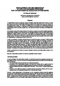
RAVE’s kinematic capabilities √ were tested with a data sample consisting of 1376 events e+ e− → W + W − → 4 jets at s = 500 GeV, generated by Pythia [5] and processed for the LDC 2007 layout [6]; the “true” W masses are plotted in Figure 1(a). Events with a mass |mW − 80.32| > 6.5 GeV are eventually discarded, retaining 1008 events. To model the expected performance of jet reconstruction in ILC experiments, the Entries 1376 Generated Monte-Carlo masses following Gaussian errors have been applied 500 to all four generated jets: √ 450 σE /E = 30%/ E (1) 400 σθ = σφ sin(θ) = 10 mrad (2) 350 The direction resolution affects the θ (polar angle) and φ (azimuth) measurements. A known general problem with the use of jets as virtual measurements is due to their compositeness: only direction and energy, but not an absolute momentum, are welldefined. However, an initialization of the jet’s momentum with its energy, followed by an appropriate inflation of the associated error, gives satisfactory results. The constraints applied are those of energy and 3-momentum conservation. They are explicitly written as (the subscripts identify the four jets): √ (3) E1 + E2 + E3 + E4 = s ~ p~1 + ~ p2 + p~3 + ~ p4 = 0 (4)

300 250 200 150 100 50 00

50 100 150 200 250 300 350 400 450 500

(a) All W masses as generated by Pythia. Entries

All combinations

2872

500 450 400 350 300

So far no distinction was made between 250 the four jets: the applied kinematic con200 straints acted equally on all final states, 150 and did not take into account which particles they could have originated from. Now 100 one has the task of associating the four jets 50 into two pairs (there are 3 possible combi00 50 100 150 200 250 300 350 400 450 500 nations), with each pair originating from a W boson decay. (b) The W masses resulting from all possible A trivial strategy is to assume that each combinations of jet association. combination is valid, and to calculate the two W masses accordingly. Figure 1(b) shows the results: each entry represents the Figure 1: Scatter plots of the W pair masses. W pair masses corresponding to one combi- The colours represent the number of entries in each bin. nation of one event.a a

About 5% of the combinations yield unphysical mass values and do not enter the plot.

LCWS/ILC 2008

A comparison of Figure 1(b) with 1(a) suggests that, as a first step, dropping combinations where both W masses exceed a pre-defined cut limit would significantly improve the performance of the association. This cut is chosen at a value of 130 GeV. For a second step, several options are feasible. A simple “equal-mass hypothesis” true negative false negative introduces in the kinematic fit, as an ad500 true positive ditional constraint, the requirement of the false positive 450 two fitted masses to be equal (because they 400 both belong to W bosons). However, such 350 a requirement would strongly favour combinations along the 45o diagonal over those 300 parallel to the axes, in contradiction to the 250 true distribution of the W pair masses as 200 shown in Figure 1(a). 150 The most obvious improvement of such a hypothesis would be to model a selection 100 requirement from two uncorrelated Breit50 Wigner (BW) distributions.b But that is 00 50 100 150 200 250 300 350 400 450 500 not possible in real-world scenarios, because the position parameter of the expected distribution is exactly the (unknown) value to Figure 2: Scatter plot of the W pair masses fitbe determined by this kinematic vertex fit. ted with the similar-mass constraint; selection Therefore, a compromise is suggested be- of the best jet association by the fit’s pseudo2 tween this idea and the “equal-mass hypoth- χ probability, applied to the reduced sample after the 130 GeV cut. esis” above [8]: The two W masses are known to not being equal, however, they are still picked from the same distribution. The likelihood of such a configuration is given by L(~ αc |~ αm , m) ¯ = L(~ αc |~ αm ) · L(m1 (~ αm ), m2 (~ αm )|m) ¯

(5)

Here, the first term holds the results of the kinematic vertex fit (parameters α~c and covariances Vc ). The second term represents the new “similar-mass hypothesis”; it models the distribution of the two masses dependent on the position parameter m, ¯ and it can be split into two symmetric terms if the masses are approximately uncorrelated. Although any p.d.f. can be used within the second term, a Gaussian model is certainly the easiest choice. Then, the objective function for the new fit can be written as T

M(~ αm , m) ¯ = [~ αm − α ~ c ] Vc−1 [~ αm − α ~ c] +

2 2 X (mi (~ αm ) − m) ¯ i=1

σt2

(6)

where σt ≈ 9 GeV is a pre-defined scale (obtained by integration over the BW). The objective function M is minimized w.r.t. α ~ m and m ¯ and yields a pseudo-χ2 , the probability of which is used as the new second step selection criterion for finding the best jet association (out of the 3 possible combinations). b

More precisely: from σ(s) =

Rs 0

LCWS/ILC 2008

dsA

s−s R A 0

dsB ρ(sA )ρ(sB ) with ρ(si ) ∝ BW(MW , ΓW , si ) [7].

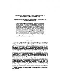
This strategy, after application Entries 1958 Mean 79.34 of the first step (130 GeV cut RMS 12.07 140 Underflow 0 mentioned above), results in 979 Overflow 2 χ / ndf 120 52.25 / 42 events; the W pair masses are Constant 133.7 ± 4.0 Mean 79.58 ± 0.27 shown in Figure 2. 100 Sigma 11.4 ± 0.2 The association performance of 80 this method is characterized by 60 type 1 and 2 errors of 1.6 % and 0.9 %, respectively. 40 Figure 3 shows the recon20 structed W masses after kine0 matic vertex fitting, including the 30 40 50 60 70 80 90 100 110 120 130 c similar-mass constraint. A Gaussian fit over the histogram range 30 . . . 130 GeV yields Figure 3: Reconstructed W masses after kinematic verfor mean and standard deviation: tex fitting with the similar-mass constraint. µ(mW ) = 79.58 ± 0.27 GeV and σ(mW ) = 11.4 ± 0.2 GeV. Scaled to 664k events expected in 4 years at the ILC (500 fb−1 , 4-jet efficiency ≈ 40%) [8], an accuracy of 0.014 GeV in determining the W mass may be achieved. 2

3

Reconstruction of Z o Z o decays

The other exemplary reconstruction was performed on a data sample of 994 Pythia events √ e+ e− → Z o Z o → 4 jets at s = 250 GeV, and processed for the LDCprime 2008 layout [9]. In contrast to the W W data of chapter 2, simulation included initial state radiation; at present, this cannot be accounted for in our kinematic reconstruction. Therefore, events with a total ZZ energy < 249 GeV are discarded, retaining 531 events. The ZZ data had the momenta of the jets correctly calculated by PFA, so they were used in this study. Apart from that, exactly the same strategies and methods as in chapter 2 have been applied. A comparison (not shown) of the reconstructed Z masses with and without kinematic constraints, respectively, reflects significant improvement.

References [1] Presentation: http://ilcagenda.linearcollider.org/contributionDisplay.py?contribId=141&sessionId=23&confId=2628

[2] [3] [4] [5] [6]

Wolfgang Waltenberger: The RAVE Repository, http://projects.hepforge.org/rave/ Kirill Prokofiev: PhD Thesis, Universit¨ at Z¨ urich, Zurich 2005. Frank Gaede: Nucl.Instr.Meth. A 559, 177 (2006). T. Sj¨ ostrand et al.: PYTHIA 6.321, http://cepa.fnal.gov/psm/simulation/mcgen/lund/ Vasiliy Morgunov (ILD Collaboration): Private communication, M-5-4 ww 500 noisr sel LDC00Sc 4.0T r1690. l2730. QGSP BERT [7] Ansgar Denner: Fortschr.Phys. 41, 307 (1993). [8] Fabian Moser: MSc Thesis, University of Technology, Vienna 2008. [9] Jenny List (ILD Collaboration): Private communication, DST01-04 ppr002 ZZ qqqq 250 LDCPrime 02Sc LCP ep+0.0 em+0.0 0001.slcio c Note that the four kinematic constraints (equ. 3 and 4) and the similar-mass constraint (equ. 6) together do not suffice to account for the redundant degrees of freedom.

LCWS/ILC 2008